はじめに
R言語で三角関数の定義や公式を可視化しようシリーズです。
この記事では、6つの三角関数のグラフを作成します。
【前の内容】
【他の記事一覧】
【この記事の内容】
円関数(三角関数)の可視化
三角関数(trigonometric functions)・円関数(circular functions)の6つの関数(sin関数・cos関数・tan関数・cot関数・sec関数・csc関数)をグラフで確認します。各関数についてはそれぞれの記事を参照してください。
(このブログでは信仰上の理由により、三角関数ではなく円関数と呼びます。)
Rを使って作図を行います。
・作図コード(クリックで展開)
利用するパッケージを読み込みます。
# 利用パッケージ
library(tidyverse)
library(gganimate)
library(patchwork)
library(magick)
この記事では、基本的にパッケージ名::関数名()の記法を使うので、パッケージを読み込む必要はありません。ただし、作図コードがごちゃごちゃしないようにパッケージ名を省略しているため、ggplot2を読み込む必要があります。
また、ネイティブパイプ演算子|>を使っています。magrittrパッケージのパイプ演算子%>%に置き換えても処理できますが、その場合はmagrittrも読み込む必要があります。
定義式の確認
まずは、4つの円関数の定義式を確認します。
円関数は、それぞれsin関数またはcos関数を用いて、次の式で定義されます。
ただし、 を整数として
のとき
なので、
は定義できません。また、
のとき
なので、
は定義できません。
は円周率で、変数
は弧度法の角度(ラジアン)です。各関数についてはそれぞれの記事「Rによる三角関数(円関数)入門:記事一覧 - からっぽのしょこ」を参照してください。
円関数の作図
次に、6つの円関数のグラフを作成します。
・作図コード(クリックで展開)
変数の範囲を指定します。
# 変数(ラジアン)の範囲を指定
theta_vec <- seq(from = -2.5*pi, to = 2.5*pi, length.out = 1000)
head(theta_vec)
## [1] -7.853982 -7.838258 -7.822534 -7.806811 -7.791087 -7.775363
曲線の座標計算用の変数(ラジアン) を作成して
theta_vecとします。円周率 は
piで扱えます。
関数曲線の描画用のデータフレームを作成します。
# 関数ラベルのレベルを指定
fnc_level_vec <- c("sin", "cos", "tan", "csc", "sec", "cot")

# 閾値を指定
threshold <- 4

# 関数曲線の座標を計算
function_curve_df <- tibble::tibble(
  t = theta_vec |>
    rep(times = length(fnc_level_vec)), # 関数の数に応じて変数を複製
  f_t = c(
    sin(theta_vec),
    cos(theta_vec),
    tan(theta_vec),
    1/sin(theta_vec),
    1/cos(theta_vec),
    1/tan(theta_vec)
  ),
  fnc = c("sin", "cos", "tan", "csc", "sec", "cot") |>
    rep(each = length(theta_vec)) |>
    factor(levels = fnc_level_vec), # 色用
  fnc_pair = c("sin", "cos", "tan", "sin", "cos", "tan") |>
    rep(each = length(theta_vec)) |>
    factor(levels = c("sin", "cos", "tan")), # 色用
  fnc_type = c("original", "original", "original", "reciprocal", "reciprocal", "reciprocal") |>
    rep(each = length(theta_vec)) # 線種用
) |>
  dplyr::mutate(
    f_t = dplyr::if_else(
      (f_t >= -threshold & f_t <= threshold), true = f_t, false = NA_real_
    ) # 閾値外の値を欠損値に置換
  )
function_curve_df
## # A tibble: 6,000 × 5
##        t    f_t fnc   fnc_pair fnc_type
##    <dbl>  <dbl> <fct> <fct>    <chr>
##  1 -7.85 -1     sin   sin      original
##  2 -7.84 -1.00  sin   sin      original
##  3 -7.82 -1.00  sin   sin      original
##  4 -7.81 -0.999 sin   sin      original
##  5 -7.79 -0.998 sin   sin      original
##  6 -7.78 -0.997 sin   sin      original
##  7 -7.76 -0.996 sin   sin      original
##  8 -7.74 -0.994 sin   sin      original
##  9 -7.73 -0.992 sin   sin      original
## 10 -7.71 -0.990 sin   sin      original
## # … with 5,990 more rows
変数 の値と関数
の値をデータフレームに格納します。csc関数は
sin()、sec関数はcos()、cot関数はtan()を使って計算できます。
や
(
は整数)付近で
または
に近付くので、閾値
thresholdを指定しておき、-threshold未満またはthresholdより大きい場合は(数値型の)欠損値NAに置き換えます。
x軸の角度目盛の描画用のベクトルを作成します。
# 半周期の目盛の数(分母の値)を指定
denom <- 2

# 目盛の通し番号(分子の値)を作成
numer_vec <- seq(
  from = floor(min(theta_vec) / pi * denom),
  to   = ceiling(max(theta_vec) / pi * denom),
  by = 1
)

# 目盛ラベル用の文字列を作成
label_vec <- paste0(c("", "-")[(numer_vec < 0)+1], "frac(", abs(numer_vec), ", ", denom, ")~pi")
head(numer_vec); head(label_vec)
## [1] -5 -4 -3 -2 -1  0
## [1] "-frac(5, 2)~pi" "-frac(4, 2)~pi" "-frac(3, 2)~pi" "-frac(2, 2)~pi"
## [5] "-frac(1, 2)~pi" "frac(0, 2)~pi"
角度(ラジアン) に関する軸目盛ラベルを
(
は整数)の形で表示することにします。
を
denomとして整数を指定します。 は、半周期
の範囲における目盛の数に対応します。
theta_vecに対して、 を
について整理した
を計算して、最小値(の小数部分を
floor()で切り捨てた値)から最大値(の小数部分をceiling()で切り上げた値)までの整数を作成してnumer_vecとします。
numer_vec, denomを使って目盛ラベル用の文字列を作成します。ギリシャ文字などの記号や数式を表示する場合は、expression()の記法を用います。オブジェクト(プログラム上の変数)の値を使う場合は、文字列として作成しておきparse()のtext引数に渡します。frac(分子, 分母)で分数、~でスペースを表示します。
漸近線の描画用のベクトルを作成します。
# 漸近線のプロット位置を作成
asymptote_even_vec <- seq(
  from = floor(min(theta_vec) / pi) + 0.5,
  to   = floor(max(theta_vec) / pi) + 0.5,
  by = 1
) * pi
asymptote_odd_vec <- seq(
  from = floor(min(theta_vec) / pi) + 1,
  to   = floor(max(theta_vec) / pi),
  by = 1
) * pi

# 漸近線の座標を格納
asymptote_df <- tibble::tibble(
  value = c(
    asymptote_even_vec,
    asymptote_odd_vec
  ),
  type = c(
    rep("even", times = length(asymptote_even_vec)),
    rep("odd", times = length(asymptote_odd_vec))
  ) # 線種用
)
asymptote_df
## # A tibble: 11 × 2
##    value type
##    <dbl> <chr>
##  1 -7.85 even
##  2 -4.71 even
##  3 -1.57 even
##  4  1.57 even
##  5  4.71 even
##  6  7.85 even
##  7 -6.28 odd
##  8 -3.14 odd
##  9  0    odd
## 10  3.14 odd
## 11  6.28 odd
(
の倍数)のとき
、
(
の倍数でない
の倍数)のとき
が発散するので、
theta_vecの範囲内の の値を(上手いこと)作成して、データフレームに格納します。
円関数のグラフを作成します。
# 軸目盛のプロット位置を計算
break_vec <- numer_vec / denom * pi

# 関数曲線を作図
curve_graph <- ggplot() +
  geom_vline(data = asymptote_df,
             mapping = aes(xintercept = value, linetype = type)) + # 漸近線
  geom_line(data = function_curve_df,
            mapping = aes(x = t, y = f_t, color = fnc), na.rm = TRUE,
            size = 1, alpha = 0.8) + # 関数曲線
  scale_x_continuous(breaks = break_vec, labels = round(break_vec, digits = 2),
                     sec.axis = sec_axis(trans = ~.,
                                         breaks = break_vec, labels = parse(text = label_vec))) + # 目盛ラベル
  scale_linetype_manual(breaks = c("even", "odd"),
                        values = c("dotdash", "twodash"),
                        labels = c(expression(i*pi), expression(frac(2*i+1, 2)*pi)),
                        name = "asymptote") + # (2種類の漸近線用)
  coord_fixed(ratio = 1) + # アスペクト比
  labs(title = "circular functions",
       color = "function",
       x = expression(theta),
       y = expression(f(theta)))
curve_graph
# 関数曲線を作図
curve_pair_graph <- ggplot() +
  geom_vline(data = asymptote_df,
             mapping = aes(xintercept = value),
             linetype = "dotdash") + # 漸近線
  geom_line(data = function_curve_df,
            mapping = aes(x = t, y = f_t, color = fnc_pair, linetype = fnc_type), na.rm = TRUE,
            size = 1, alpha = 0.8) + # 関数曲線
  scale_x_continuous(breaks = break_vec, labels = round(break_vec, digits = 2),
                     sec.axis = sec_axis(trans = ~.,
                                         breaks = break_vec, labels = parse(text = label_vec))) + # 目盛ラベル
  scale_linetype_manual(breaks = c("original", "reciprocal"),
                        values = c("solid", "dashed"),
                        labels = c(expression(f(x)), expression(frac(1, f(x)))),
                        name = "function") + # (2種類の漸近線用)
  coord_fixed(ratio = 1) + # アスペクト比
  labs(title = "circular functions",
       color = "function",
       x = expression(theta),
       y = expression(f(theta)))
curve_pair_graph


x軸を変数(ラジアン) 、y軸を各関数
として曲線を描画します。また、基本となる関数
を実線、それぞれの逆数
を破線で示します。
x軸が の点(
の前後
間隔)
の点(
の前後
間隔)に漸近線を破線で描画します。
元の関数と逆数とで何となくひっくり返したような形で、元の関数が0のとき漸近線(不連続)になるのが分かります。
単位円の作図
続いて、円関数の可視化に利用する単位円(unit circle)のグラフを確認します。円やラジアン(弧度法の角度)、度数法と弧度法の関係については「【R】円周の作図 - からっぽのしょこ」を参照してください。
・作図コード(クリックで展開)
単位円の描画用のデータフレームを作成します。
# 半径を指定
r <- 1

# 円周の座標を計算
circle_df <- tibble::tibble(
  t = seq(from = 0, to = 2*pi, length.out = 601), # ラジアン
  x = r * cos(t),
  y = r * sin(t)
)
circle_df
## # A tibble: 601 × 3
##         t     x      y
##     <dbl> <dbl>  <dbl>
##  1 0      1     0
##  2 0.0105 1.00  0.0105
##  3 0.0209 1.00  0.0209
##  4 0.0314 1.00  0.0314
##  5 0.0419 0.999 0.0419
##  6 0.0524 0.999 0.0523
##  7 0.0628 0.998 0.0628
##  8 0.0733 0.997 0.0732
##  9 0.0838 0.996 0.0837
## 10 0.0942 0.996 0.0941
## # … with 591 more rows
単位円の円周の座標計算用のラジアンとして の範囲の値を作成して、x軸の値
とy軸の値
を計算します。
角度目盛の描画用のデータフレームを作成します。
# 半円の目盛の数(分母の値)を指定
denom <- 6

# 角度目盛の描画用
d <- 1.1
radian_lable_df <- tibble::tibble(
  nomer = seq(from = 0, to = 2*denom-1, by = 1), # 目盛の通し番号(分子の値)を作成
  t_deg = nomer / denom * 180, # 度数法
  t_rad = nomer / denom * pi,  # 弧度法
  x = r * cos(t_rad),
  y = r * sin(t_rad),
  label_x = d * x,
  label_y = d * y,
  rad_label = paste0("frac(", nomer, ", ", denom, ")~pi"), # ラジアンラベル
  h = 1 - (x * 0.5 + 0.5),
  v = 1 - (y * 0.5 + 0.5)
)
radian_lable_df
## # A tibble: 12 × 10
##    nomer t_deg t_rad         x         y   label_x   label_y rad_label         h
##    <dbl> <dbl> <dbl>     <dbl>     <dbl>     <dbl>     <dbl> <chr>         <dbl>
##  1     0     0 0      1   e+ 0  0         1.1 e+ 0  0        frac(0, 6)~… 0
##  2     1    30 0.524  8.66e- 1  5   e- 1  9.53e- 1  5.5 e- 1 frac(1, 6)~… 0.0670
##  3     2    60 1.05   5   e- 1  8.66e- 1  5.5 e- 1  9.53e- 1 frac(2, 6)~… 0.25
##  4     3    90 1.57   6.12e-17  1   e+ 0  6.74e-17  1.1 e+ 0 frac(3, 6)~… 0.5
##  5     4   120 2.09  -5   e- 1  8.66e- 1 -5.5 e- 1  9.53e- 1 frac(4, 6)~… 0.75
##  6     5   150 2.62  -8.66e- 1  5   e- 1 -9.53e- 1  5.5 e- 1 frac(5, 6)~… 0.933
##  7     6   180 3.14  -1   e+ 0  1.22e-16 -1.1 e+ 0  1.35e-16 frac(6, 6)~… 1
##  8     7   210 3.67  -8.66e- 1 -5   e- 1 -9.53e- 1 -5.5 e- 1 frac(7, 6)~… 0.933
##  9     8   240 4.19  -5.00e- 1 -8.66e- 1 -5.50e- 1 -9.53e- 1 frac(8, 6)~… 0.75
## 10     9   270 4.71  -1.84e-16 -1   e+ 0 -2.02e-16 -1.1 e+ 0 frac(9, 6)~… 0.5
## 11    10   300 5.24   5   e- 1 -8.66e- 1  5.5 e- 1 -9.53e- 1 frac(10, 6)… 0.25
## 12    11   330 5.76   8.66e- 1 -5.00e- 1  9.53e- 1 -5.50e- 1 frac(11, 6)… 0.0670
## # … with 1 more variable: v <dbl>
目盛指示線や目盛グリッド用の座標をx, y列、目盛ラベル用の座標をlabel_x, label_y列とします。ラベルの表示位置をdで調整します。
円周と角度目盛のグラフを作成します。
# グラフサイズを指定
axis_size <- 1.5

# 円周を作図
circle_graph <- ggplot() +
  geom_path(data = circle_df,
            mapping = aes(x = x, y = y),
            size = 1) + # 円周
  geom_segment(data = radian_lable_df,
               mapping = aes(x = 0, y = 0, xend = x, yend = y),
               linetype = "dotted") + # 角度目盛グリッド
  geom_text(data = radian_lable_df,
            mapping = aes(x = x, y = y, angle = t_deg+90),
            label = "|", size = 2) + # 角度目盛指示線
  geom_text(data = radian_lable_df,
            mapping = aes(x = label_x, y = label_y, label = rad_label,
                          hjust = h, vjust = v), parse = TRUE) + # 角度目盛ラベル
  coord_fixed(ratio = 1,
              xlim = c(-axis_size, axis_size), ylim = c(-axis_size, axis_size)) + # 描画領域
  labs(title = "unit circle",
       subtitle = parse(text = paste0("r==", r)),
       x = expression(x == r~cos~theta),
       y = expression(y == r~sin~theta))
circle_graph

このグラフ上に円関数の値を直線として描画します。
なす角と円関数の関係
次は、単位円上におけるなす角と円関数(sin・cos・tan・cot・sec・csc)の関係をグラフで可視化します。関数の値を線分の長さと座標の正負に対応させます。
グラフの作成
変数を固定した円関数をグラフで確認します。
・作図コード(クリックで展開)
変数の値を指定して、円周上の点の描画用のデータフレームを作成します。
# なす角(変数)を指定
theta <- 1/6 * pi

# 単位円上の点の座標を計算
point_df <- tibble::tibble(
  t = theta,
  sin_t = sin(theta),
  cos_t = cos(theta)
)
point_df
## # A tibble: 1 × 3
##       t sin_t cos_t
##   <dbl> <dbl> <dbl>
## 1 0.524   0.5 0.866
単位円におけるなす角(ラジアン) を
thetaとして値を指定します。ただし、thetaが0のとき、計算結果にInfや-Infが含まれるため、意図しないグラフになります(理論上はpiなどのときにも発散しますが、プログラム上の誤差によりInfになりません)。発散時の対策については「アニメーションの作成」を参照してください。
の値と
の値をデータフレームに格納します。
なす角マークの描画用のデータフレームを作成します。
# なす角マークの座標を計算
d <- 0.15
angle_mark_df <- tibble::tibble(
  t = seq(from = 0, to = theta, length.out = 100),
  x = d * cos(t),
  y = d * sin(t)
)
angle_mark_df
## # A tibble: 100 × 3
##          t     x        y
##      <dbl> <dbl>    <dbl>
##  1 0       0.15  0
##  2 0.00529 0.150 0.000793
##  3 0.0106  0.150 0.00159
##  4 0.0159  0.150 0.00238
##  5 0.0212  0.150 0.00317
##  6 0.0264  0.150 0.00397
##  7 0.0317  0.150 0.00476
##  8 0.0370  0.150 0.00555
##  9 0.0423  0.150 0.00634
## 10 0.0476  0.150 0.00714
## # … with 90 more rows
なす角 を示すなす角マークを描画するために、
のラジアンを作成して、円弧の座標を計算します。サイズの調整用の値(半径)を
dとします。
なす角ラベルの描画用のデータフレームを作成します。
# なす角ラベルの座標を計算
d <- 0.21
angle_label_df <- tibble::tibble(
  t = 0.5 * theta,
  x = d * cos(t),
  y = d * sin(t)
)
angle_label_df
## # A tibble: 1 × 3
##       t     x      y
##   <dbl> <dbl>  <dbl>
## 1 0.262 0.203 0.0544
なす角マークの中点にラベルを配置するために、 のラジアンを作成して、円弧上の点の座標を計算します。表示位置の調整用の値(原点からのノルム)を
dとします。
ここまでは、共通の処理です。ここからは、2つの方法で図示します。
パターン1
1つ目の方法では、原点と円周上の点を結ぶ線分を斜辺として各関数を可視化します。
・作図コード(クリックで展開)
半径と円関数を示す線分の描画用のデータフレームを作成します。
# 関数ラベルのレベルを指定
fnc_level_vec <- c("r", "sin", "cos", "tan", "cot", "sec", "csc")

# 反転フラグを設定
sin_flag <- sin(theta) >= 0
cos_flag <- cos(theta) >= 0

# 関数直線の線分の座標を計算
function_line_df <- tibble::tibble(
  fnc = c(
    "r", "r", "r", "r", "r",
    "sin", "sin",
    "cos", "cos",
    "tan", "tan",
    "cot", "cot", "cot", "cot",
    "sec", "sec",
    "csc", "csc"
  ) |>
    factor(levels = fnc_level_vec), # 色用
  x_from = c(
    0, 0, 1/tan(theta), ifelse(test = cos_flag, yes = NA, no = -1/tan(theta)), 0,
    0, cos(theta),
    0, 0,
    1, ifelse(test = sin_flag, yes = NA, no = 1),
    0, 0, ifelse(test = cos_flag, yes = NA, no = 0), ifelse(test = cos_flag, yes = NA, no = 0),
    0, ifelse(test = sin_flag, yes = NA, no = 0),
    0, ifelse(test = cos_flag, yes = NA, no = 0)
  ),
  y_from = c(
    0, 0, 0, ifelse(test = cos_flag, yes = NA, no = 0), 0,
    0, 0,
    0, sin(theta),
    0, ifelse(test = sin_flag, yes = NA, no = 0),
    0, 1, ifelse(test = cos_flag, yes = NA, no = 0), ifelse(test = cos_flag, yes = NA, no = 1),
    0, ifelse(test = sin_flag, yes = NA, no = 0),
    0, ifelse(test = cos_flag, yes = NA, no = 0)
  ),
  x_to = c(
    1, cos(theta), 1/tan(theta), ifelse(test = cos_flag, yes = NA, no = -1/tan(theta)), 0,
    0, cos(theta),
    cos(theta), cos(theta),
    1, ifelse(test = sin_flag, yes = NA, no = 1),
    1/tan(theta), 1/tan(theta), ifelse(test = cos_flag, yes = NA, no = -1/tan(theta)), ifelse(test = cos_flag, yes = NA, no = -1/tan(theta)),
    1, ifelse(test = sin_flag, yes = NA, no = 1),
    ifelse(test = cos_flag, yes = 1/tan(theta), no = -1/tan(theta)), ifelse(test = cos_flag, yes = NA, no = 1/tan(theta))
  ),
  y_to = c(
    0, sin(theta), 1, ifelse(test = cos_flag, yes = NA, no = 1), 1,
    sin(theta), sin(theta),
    0, sin(theta),
    tan(theta), ifelse(test = sin_flag, yes = NA, no = -tan(theta)),
    0, 1, ifelse(test = cos_flag, yes = NA, no = 0), ifelse(test = cos_flag, yes = NA, no = 1),
    ifelse(test = sin_flag, yes = tan(theta), no = -tan(theta)), ifelse(test = sin_flag, yes = NA, no = tan(theta)),
    1, ifelse(test = cos_flag, yes = NA, no = 1)
  ),
  width = c(
    "normal", "normal", "thin", "thin", "thin",
    "normal", "normal",
    "bold", "normal",
    "normal", "normal",
    "thin", "normal", "thin", "normal",
    "bold", "bold",
    "thin", "thin"
  ), # 太さ用
  type = c(
    "main", "main", "sub", "sub", "sub",
    "main", "main",
    "main", "main",
    "main", "sub",
    "main", "main", "sub", "sub",
    "main", "sub",
    "main", "sub"
  ) # 線種用
)
function_line_df
## # A tibble: 19 × 7
##    fnc   x_from y_from   x_to   y_to width  type
##    <fct>  <dbl>  <dbl>  <dbl>  <dbl> <chr>  <chr>
##  1 r      0        0    1      0     normal main
##  2 r      0        0    0.866  0.5   normal main
##  3 r      1.73     0    1.73   1     thin   sub
##  4 r     NA       NA   NA     NA     thin   sub
##  5 r      0        0    0      1     thin   sub
##  6 sin    0        0    0      0.5   normal main
##  7 sin    0.866    0    0.866  0.5   normal main
##  8 cos    0        0    0.866  0     bold   main
##  9 cos    0        0.5  0.866  0.5   normal main
## 10 tan    1        0    1      0.577 normal main
## 11 tan   NA       NA   NA     NA     normal sub
## 12 cot    0        0    1.73   0     thin   main
## 13 cot    0        1    1.73   1     normal main
## 14 cot   NA       NA   NA     NA     thin   sub
## 15 cot   NA       NA   NA     NA     normal sub
## 16 sec    0        0    1      0.577 bold   main
## 17 sec   NA       NA   NA     NA     bold   sub
## 18 csc    0        0    1.73   1     thin   main
## 19 csc   NA       NA   NA     NA     thin   sub
関数を区別するためのfnc列の因子レベルをfnc_level_vecとして指定しておきます。因子レベルは、線分の描画順(重なり順)や色付け順に影響します。
各線分の始点の座標をx_from, y_from列、終点の座標をx_to, y_to列として、完成図を見ながら頑張って指定します。詳しくはそれぞれの関数の記事を参照してください。
関数名(ラベル)の描画用のデータフレームを作成します。
# 関数ラベルの座標を計算
function_label_df <- tibble::tibble(
  fnc = c(
    "sin",
    "cos",
    "tan", "tan",
    "cot", "cot",
    "sec", "sec",
    "csc", "csc"
  ) |>
    factor(levels = fnc_level_vec), # 色用
  x = c(
    0,
    0.5 * cos(theta),
    1, ifelse(test = sin_flag, yes = NA, no = 1),
    0.5 / tan(theta), ifelse(test = cos_flag, yes = NA, no = -0.5/tan(theta)),
    0.5, ifelse(test = sin_flag, yes = NA, no = 0.5),
    0.5 / ifelse(test = cos_flag, yes = tan(theta), no = -tan(theta)), ifelse(test = cos_flag, yes = NA, no = 0.5/tan(theta))
  ),
  y = c(
    0.5 * sin(theta),
    0,
    0.5 * tan(theta), ifelse(test = sin_flag, yes = NA, no = -0.5*tan(theta)),
    1, ifelse(test = cos_flag, yes = NA, no = 1),
    0.5 * ifelse(test = sin_flag, yes = tan(theta), no = -tan(theta)), ifelse(test = sin_flag, yes = NA, no = 0.5*tan(theta)),
    0.5, ifelse(test = cos_flag, yes = NA, no = 0.5)
  ),
  angle = c(
    90,
    0,
    90, 90,
    0, 0,
    0, 0,
    0, 0
  ),
  h = c(
    0.5,
    0.5,
    0.5, 0.5,
    0.5, 0.5,
    1.2, 1.2,
    -0.2,-0.2
  ),
  v = c(
    -0.5,
    1,
    1, 1,
    -0.5, -0.5,
    0.5, 0.5,
    0.5, 0.5
  ),
  fnc_label = c(
    "sin~theta",
    "cos~theta",
    "tan~theta", "-tan~theta",
    "cot~theta", "-cot~theta",
    "sec~theta", "-sec~theta",
    "csc~theta", "-csc~theta"
  ) # 関数ラベル
)
function_label_df
## # A tibble: 10 × 7
##    fnc        x      y angle     h     v fnc_label
##    <fct>  <dbl>  <dbl> <dbl> <dbl> <dbl> <chr>
##  1 sin    0      0.25     90   0.5  -0.5 sin~theta
##  2 cos    0.433  0         0   0.5   1   cos~theta
##  3 tan    1      0.289    90   0.5   1   tan~theta
##  4 tan   NA     NA        90   0.5   1   -tan~theta
##  5 cot    0.866  1         0   0.5  -0.5 cot~theta
##  6 cot   NA     NA         0   0.5  -0.5 -cot~theta
##  7 sec    0.5    0.289     0   1.2   0.5 sec~theta
##  8 sec   NA     NA         0   1.2   0.5 -sec~theta
##  9 csc    0.866  0.5       0  -0.2   0.5 csc~theta
## 10 csc   NA     NA         0  -0.2   0.5 -csc~theta
この例では、関数を示す線分の中点に関数名を表示するため、中点の座標とラベル用の文字列などを格納します。
ラベルの表示角度をangle列、表示角度に応じた左右の表示位置をh列、上下の表示位置をv列として値を指定します。
変数と関数の値(ラベル)の表示用の文字列を作成します。
# 変数ラベル用の文字列を作成
variable_label <- paste0(
  "list(",
  "theta==", round(theta/pi, digits = 2), "*pi",
  ", sin~theta==", round(sin(theta), digits = 2),
  ", cos~theta==", round(cos(theta), digits = 2),
  ", tan~theta==", round(tan(theta), digits = 2),
  ", cot~theta==", round(1/tan(theta), digits = 2),
  ", sec~theta==", round(1/cos(theta), digits = 2),
  ", csc~theta==", round(1/sin(theta), digits = 2),
  ")"
)
variable_label
## [1] "list(theta==0.17*pi, sin~theta==0.5, cos~theta==0.87, tan~theta==0.58, cot~theta==1.73, sec~theta==1.15, csc~theta==2)"
==で等号、list(変数1, 変数2)で複数の(数式上の)変数を並べて表示します。(プログラム上の)変数の値を使う場合は、文字列として作成しておきparse()のtext引数に渡します。
単位円上に円関数の線分を重ねたグラフを作成します。
# グラフサイズ用の値を設定
axis_lower <- 1.5
x_min <- min(-axis_lower, 1/tan(theta))
x_max <- max(axis_lower, 1/tan(theta))
y_min <- min(-axis_lower, tan(theta))
y_max <- max(axis_lower, tan(theta))

# 単位円上に関数直線を作図
fnc_line_graph <- ggplot() +
  geom_segment(data = radian_lable_df,
               mapping = aes(x = 0, y = 0, xend = x, yend = y),
               color = "white") + # 角度目盛グリッド
  geom_text(data = radian_lable_df,
            mapping = aes(x = x, y = y, angle = t_deg+90), label = "|",
            size = 2) + # 角度目盛指示線
  geom_text(data = radian_lable_df,
            mapping = aes(x = label_x, y = label_y, label = rad_label,
                          hjust = h, vjust = v), parse = TRUE) + # 角度目盛ラベル
  geom_path(data = angle_mark_df,
            mapping = aes(x = x, y = y),
            size = 0.5) + # なす角マーク
  geom_text(data = angle_label_df,
            mapping = aes(x = x, y = y), label = "theta", parse = TRUE,
            size = 5) + # なす角ラベル
  geom_path(data = circle_df,
            mapping = aes(x = x, y = y),
            size = 1) + # 円周
  geom_point(data = point_df,
             mapping = aes(x = cos_t, y = sin_t),
             size = 4) + # 円周上の点
  geom_hline(yintercept = 1, linetype = "dashed") + # 補助線
  geom_vline(xintercept = 1, linetype = "dashed") + # 補助線
  geom_segment(data = function_line_df,
               mapping = aes(x = x_from, y = y_from, xend = x_to, yend = y_to,
                             color = fnc, size = width, linetype = type), na.rm = TRUE) + # 関数直線
  geom_text(data = function_label_df,
            mapping = aes(x = x, y = y, label = fnc_label, color = fnc,
                          hjust = h, vjust = v, angle = angle),
            parse = TRUE, na.rm = TRUE, show.legend = FALSE) + # 関数ラベル
  scale_color_manual(breaks = fnc_level_vec,
                     values = c("black", scales::hue_pal()(length(fnc_level_vec)-1))) + # (半径直線を黒色にしたい)
  scale_size_manual(breaks = c("normal", "bold", "thin"),
                    values = c(1, 1.6, 0.8), guide = "none") + # (線が重なる対策)
  scale_linetype_manual(breaks = c("main", "sub"),
                        values = c("solid", "twodash"), guide = "none") + # (補助線を描き分けたい)
  coord_fixed(ratio = 1,
              xlim = c(x_min, x_max), ylim = c(y_min, y_max)) + # 描画領域
  labs(title = "circular functions",
       subtitle = parse(text = variable_label),
       color = "function",
       x = "x", y = "y")
fnc_line_graph
geom_segment()で線分を描画して、各関数の値を直線で示します。
geom_label()でラベル(文字列)を描画します。

「x軸線の正の部分(原点 と点
を結ぶ線分)」と「原点と円周上の点を結ぶ線分」のなす角を
とします。単位円の円周上の点の座標は
なので、sin関数はy軸の値(高さ)、cos関数はx軸の値(横幅)に対応します。他の関数についても円周上の点(なす角)によって決まります。詳しくはそれぞれの関数の記事を参照してください。
パターン2
2つ目の方法では、原点と円周上の点を結ぶ線分を底辺として各関数を可視化します。
・作図コード(クリックで展開)
半径と円関数を示す線分の描画用のデータフレームを作成します。
# 関数直線の線分の座標を計算
function_line_df <- tibble::tibble(
  fnc = c(
    "r", "r",
    "sin",
    "cos",
    "tan",
    "cot",
    "sec",
    "csc"
  ) |>
    factor(levels = fnc_level_vec), # 色用
  x_from = c(
    0, 0,
    cos(theta),
    0,
    cos(theta),
    cos(theta),
    0,
    0
  ),
  y_from = c(
    0, 0,
    0,
    sin(theta),
    sin(theta),
    sin(theta),
    0,
    0
  ),
  x_to = c(
    1, cos(theta),
    cos(theta),
    cos(theta),
    1/cos(theta),
    0,
    1/cos(theta),
    0
  ),
  y_to = c(
    0, sin(theta),
    sin(theta),
    sin(theta),
    0,
    1/sin(theta),
    0,
    1/sin(theta)
  )
)
function_line_df
## # A tibble: 8 × 5
##   fnc   x_from y_from  x_to  y_to
##   <fct>  <dbl>  <dbl> <dbl> <dbl>
## 1 r      0        0   1       0
## 2 r      0        0   0.866   0.5
## 3 sin    0.866    0   0.866   0.5
## 4 cos    0        0.5 0.866   0.5
## 5 tan    0.866    0.5 1.15    0
## 6 cot    0.866    0.5 0       2
## 7 sec    0        0   1.15    0
## 8 csc    0        0   0       2
「パターン1」のときと同様に、半径と関数の線分の座標を格納します。
関数名(ラベル)の描画用のデータフレームを作成します。
# 関数ラベルの座標を計算
function_label_df <- tibble::tibble(
  fnc = c("sin", "cos", "tan", "cot", "sec", "csc") |>
    factor(levels = fnc_level_vec), # 色用
  x = c(
    cos(theta),
    0.5 * cos(theta),
    0.5 * (1/cos(theta) + cos(theta)),
    0.5 * cos(theta),
    0.5 / cos(theta),
    0
  ),
  y = c(
    0.5 * sin(theta),
    sin(theta),
    0.5 * sin(theta),
    0.5 * (1/sin(theta) + sin(theta)),
    0,
    0.5 / sin(theta)
  ),
  angle = c(90, 0, 0, 0, 0, 90),
  h = c(0.5, 0.5, -0.2, -0.2, 0.5, 0.5),
  v = c(-0.5, -0.5, 0.5, 0.5, 1, 1),
  fnc_label = c("sin~theta", "cos~theta", "tan~theta", "cot~theta", "sec~theta", "csc~theta") # 関数ラベル
)
function_label_df
## # A tibble: 6 × 7
##   fnc       x     y angle     h     v fnc_label
##   <fct> <dbl> <dbl> <dbl> <dbl> <dbl> <chr>
## 1 sin   0.866  0.25    90   0.5  -0.5 sin~theta
## 2 cos   0.433  0.5      0   0.5  -0.5 cos~theta
## 3 tan   1.01   0.25     0  -0.2   0.5 tan~theta
## 4 cot   0.433  1.25     0  -0.2   0.5 cot~theta
## 5 sec   0.577  0        0   0.5   1   sec~theta
## 6 csc   0      1       90   0.5   1   csc~theta
線分の中点の座標とラベル用の文字列などを格納します。
単位円上に円関数の線分を重ねたグラフを作成します。
# グラフサイズ用の値を設定
axis_lower <- 1.5
x_min <- min(-axis_lower, 1/cos(theta))
x_max <- max(axis_lower, 1/cos(theta))
y_min <- min(-axis_lower, 1/sin(theta))
y_max <- max(axis_lower, 1/sin(theta))

# 単位円上に関数直線を作図
fnc_line_graph <- ggplot() +
  geom_segment(data = radian_lable_df,
               mapping = aes(x = 0, y = 0, xend = x, yend = y),
               color = "white") + # 角度目盛グリッド
  geom_text(data = radian_lable_df,
            mapping = aes(x = x, y = y, angle = t_deg+90), label = "|",
            size = 2) + # 角度目盛指示線
  geom_text(data = radian_lable_df,
            mapping = aes(x = label_x, y = label_y, label = rad_label,
                          hjust = h, vjust = v), parse = TRUE) + # 角度目盛ラベル
  geom_path(data = angle_mark_df,
            mapping = aes(x = x, y = y),
            size = 0.5) + # なす角マーク
  geom_text(data = angle_label_df,
            mapping = aes(x = x, y = y), label = "theta", parse = TRUE,
            size = 5) + # なす角ラベル
  geom_path(data = circle_df,
            mapping = aes(x = x, y = y),
            size = 1) + # 円周
  geom_point(data = point_df,
             mapping = aes(x = cos_t, y = sin_t),
             size = 4) + # 円周上の点
  geom_hline(yintercept = 0, linetype = "dashed") + # 補助線
  geom_vline(xintercept = 0, linetype = "dashed") + # 補助線
  geom_segment(data = function_line_df,
               mapping = aes(x = x_from, y = y_from, xend = x_to, yend = y_to, color = fnc),
               size = 1) + # 関数直線
  geom_text(data = function_label_df,
            mapping = aes(x = x, y = y, label = fnc_label, color = fnc,
                          hjust = h, vjust = v, angle = angle),
            parse = TRUE, show.legend = FALSE) + # 関数ラベル
  scale_color_manual(breaks = fnc_level_vec,
                     values = c("black", scales::hue_pal()(length(fnc_level_vec)-1))) + # (半径直線を黒色にしたい)
  coord_fixed(ratio = 1,
              xlim = c(x_min, x_max), ylim = c(y_min, y_max)) + # 描画領域
  labs(title = "circular functions",
       subtitle = parse(text = variable_label),
       color = "function",
       x = "x", y = "y")
fnc_line_graph

こちらの図は、原点と点 を結ぶ線分を底辺、x軸線やy軸線の一部を斜辺としたときのパターン1の図と言えます。文字通り首を捻って見てください。相似関係が分かりやすいように補助線を入れた図については、それぞれの関数の記事を参照してください。
アニメーションの作成
続いて、変数の値を変化させた円関数をアニメーションで確認します。
・作図コード(クリックで展開)
フレーム数を指定して、変数として用いる値を作成します。
# フレーム数を指定
frame_num <- 180

# なす角(変数)の範囲を指定
theta_i <- seq(from = -2*pi, to = 2*pi, length.out = frame_num+1)[1:frame_num]
head(theta_i)
## [1] -6.283185 -6.213372 -6.143559 -6.073746 -6.003933 -5.934119
フレーム数frame_numを指定して、単位円におけるなす角(ラジアン) の値を等間隔に
frame_num個作成します。最小値(form引数)と最大値(to引数)の範囲を の倍数にし
frame_num + 1個の等間隔の値を作成して、最後の値を除くと最後のフレームと最初のフレームのグラフが繋がります。
フレーム切替用のラベルの文字列ベクトルを作成します。
# 変数ラベル用の文字列を作成
frame_label_vec <- paste0(
  "θ = ", round(theta_i/pi, digits = 2), " π",
  ", sin θ = ", round(sin(theta_i), digits = 2),
  ", cos θ = ", round(cos(theta_i), digits = 2),
  ", tan θ = ", round(tan(theta_i), digits = 2),
  ", cot θ = ", round(1/tan(theta_i), digits = 2),
  ", sec θ = ", round(1/cos(theta_i), digits = 2),
  ", csc θ = ", round(1/sin(theta_i), digits = 2)
)
head(frame_label_vec)
## [1] "θ = -2 π, sin θ = 0, cos θ = 1, tan θ = 0, cot θ = 4082809838298843, sec θ = 1, csc θ = 4082944682095961"
## [2] "θ = -1.98 π, sin θ = 0.07, cos θ = 1, tan θ = 0.07, cot θ = 14.3, sec θ = 1, csc θ = 14.34"
## [3] "θ = -1.96 π, sin θ = 0.14, cos θ = 0.99, tan θ = 0.14, cot θ = 7.12, sec θ = 1.01, csc θ = 7.19"
## [4] "θ = -1.93 π, sin θ = 0.21, cos θ = 0.98, tan θ = 0.21, cot θ = 4.7, sec θ = 1.02, csc θ = 4.81"
## [5] "θ = -1.91 π, sin θ = 0.28, cos θ = 0.96, tan θ = 0.29, cot θ = 3.49, sec θ = 1.04, csc θ = 3.63"
## [6] "θ = -1.89 π, sin θ = 0.34, cos θ = 0.94, tan θ = 0.36, cot θ = 2.75, sec θ = 1.06, csc θ = 2.92"
この例では、フレームごとの変数と関数の値を表示するために、theta_iを用いた文字列をフレーム切替用のラベル列として使います。フレーム番号として、通し番号を用いても作図できます。
円周上の点の描画用のデータフレームを作成します。
# 単位円上の点の座標を計算
anim_point_df <- tibble::tibble(
  t = theta_i,
  sin_t = sin(theta_i),
  cos_t = cos(theta_i),
  frame_label = factor(frame_label_vec, levels = frame_label_vec) # フレーム切替用ラベル
)
anim_point_df
## # A tibble: 180 × 4
##        t    sin_t cos_t frame_label
##    <dbl>    <dbl> <dbl> <fct>
##  1 -6.28 2.45e-16 1     θ = -2 π, sin θ = 0, cos θ = 1, tan θ = 0, cot θ …
##  2 -6.21 6.98e- 2 0.998 θ = -1.98 π, sin θ = 0.07, cos θ = 1, tan θ = 0.07…
##  3 -6.14 1.39e- 1 0.990 θ = -1.96 π, sin θ = 0.14, cos θ = 0.99, tan θ = 0…
##  4 -6.07 2.08e- 1 0.978 θ = -1.93 π, sin θ = 0.21, cos θ = 0.98, tan θ = 0…
##  5 -6.00 2.76e- 1 0.961 θ = -1.91 π, sin θ = 0.28, cos θ = 0.96, tan θ = 0…
##  6 -5.93 3.42e- 1 0.940 θ = -1.89 π, sin θ = 0.34, cos θ = 0.94, tan θ = 0…
##  7 -5.86 4.07e- 1 0.914 θ = -1.87 π, sin θ = 0.41, cos θ = 0.91, tan θ = 0…
##  8 -5.79 4.69e- 1 0.883 θ = -1.84 π, sin θ = 0.47, cos θ = 0.88, tan θ = 0…
##  9 -5.72 5.30e- 1 0.848 θ = -1.82 π, sin θ = 0.53, cos θ = 0.85, tan θ = 0…
## 10 -5.65 5.88e- 1 0.809 θ = -1.8 π, sin θ = 0.59, cos θ = 0.81, tan θ = 0.…
## # … with 170 more rows
の値と
の値をフレームラベルと共に格納します。
なす角マークの描画用のデータフレームを作成します。
# なす角マークの座標を計算
d <- 0.15
anim_angle_mark_df <- tibble::tibble(
  frame_i = 1:frame_num # フレーム番号
) |>
  dplyr::group_by(frame_i) |> # ラジアンの作成用
  dplyr::summarise(
    t = seq(from = 0, to = theta_i[frame_i], length.out = 100), .groups = "drop"
  ) |> # なす角以下のラジアンを作成
  dplyr::mutate(
    x = d * cos(t),
    y = d * sin(t),
    frame_label = frame_label_vec[frame_i] |>
      factor(levels = frame_label_vec) # フレーム切替用ラベル
  )
anim_angle_mark_df
## # A tibble: 18,000 × 5
##    frame_i       t     x        y frame_label
##      <int>   <dbl> <dbl>    <dbl> <fct>
##  1       1  0      0.15   0       θ = -2 π, sin θ = 0, cos θ = 1, tan θ = …
##  2       1 -0.0635 0.150 -0.00951 θ = -2 π, sin θ = 0, cos θ = 1, tan θ = …
##  3       1 -0.127  0.149 -0.0190  θ = -2 π, sin θ = 0, cos θ = 1, tan θ = …
##  4       1 -0.190  0.147 -0.0284  θ = -2 π, sin θ = 0, cos θ = 1, tan θ = …
##  5       1 -0.254  0.145 -0.0377  θ = -2 π, sin θ = 0, cos θ = 1, tan θ = …
##  6       1 -0.317  0.143 -0.0468  θ = -2 π, sin θ = 0, cos θ = 1, tan θ = …
##  7       1 -0.381  0.139 -0.0557  θ = -2 π, sin θ = 0, cos θ = 1, tan θ = …
##  8       1 -0.444  0.135 -0.0645  θ = -2 π, sin θ = 0, cos θ = 1, tan θ = …
##  9       1 -0.508  0.131 -0.0729  θ = -2 π, sin θ = 0, cos θ = 1, tan θ = …
## 10       1 -0.571  0.126 -0.0811  θ = -2 π, sin θ = 0, cos θ = 1, tan θ = …
## # … with 17,990 more rows
フレーム番号(とフレームラベル)を格納しフレーム列でグループ化して、フレーム(変数の値)ごとにsummarise()を使って0からなす角theta_n[frame_i]までの値(ラジアン)を作成して、円弧の座標を計算します。
なす角ラベルの描画用のデータフレームを作成します。
# なす角ラベルの座標を計算
d <- 0.21
anim_angle_label_df <- tibble::tibble(
  frame_i = 1:frame_num, # フレーム番号
  t = 0.5 * theta_i,
  x = d * cos(t),
  y = d * sin(t),
  frame_label = factor(frame_label_vec, levels = frame_label_vec) # フレーム切替用ラベル
)
anim_angle_label_df
## # A tibble: 180 × 5
##    frame_i     t      x         y frame_label
##      <int> <dbl>  <dbl>     <dbl> <fct>
##  1       1 -3.14 -0.21  -2.57e-17 θ = -2 π, sin θ = 0, cos θ = 1, tan θ = …
##  2       2 -3.11 -0.210 -7.33e- 3 θ = -1.98 π, sin θ = 0.07, cos θ = 1, tan…
##  3       3 -3.07 -0.209 -1.46e- 2 θ = -1.96 π, sin θ = 0.14, cos θ = 0.99, …
##  4       4 -3.04 -0.209 -2.20e- 2 θ = -1.93 π, sin θ = 0.21, cos θ = 0.98, …
##  5       5 -3.00 -0.208 -2.92e- 2 θ = -1.91 π, sin θ = 0.28, cos θ = 0.96, …
##  6       6 -2.97 -0.207 -3.65e- 2 θ = -1.89 π, sin θ = 0.34, cos θ = 0.94, …
##  7       7 -2.93 -0.205 -4.37e- 2 θ = -1.87 π, sin θ = 0.41, cos θ = 0.91, …
##  8       8 -2.90 -0.204 -5.08e- 2 θ = -1.84 π, sin θ = 0.47, cos θ = 0.88, …
##  9       9 -2.86 -0.202 -5.79e- 2 θ = -1.82 π, sin θ = 0.53, cos θ = 0.85, …
## 10      10 -2.83 -0.200 -6.49e- 2 θ = -1.8 π, sin θ = 0.59, cos θ = 0.81, t…
## # … with 170 more rows
フレームごとに、なす角マークの中点にラベルを配置するように、円弧上の点の座標を計算します。
ここまでは、共通の処理です。ここからは、「グラフの作成」のときと同様に2つの方法で図示します。
パターン1
・作図コード(クリックで展開)
半径と円関数を示す線分の描画用のデータフレームを作成します。
# 関数ラベルのレベルを指定
fnc_level_vec <- c("r", "sin", "cos", "tan", "cot", "sec", "csc")

# 反転フラグを設定
sin_flag_i <- sin(theta_i) >= 0
cos_flag_i <- cos(theta_i) >= 0

# 関数直線の線分の座標を計算
anim_function_line_df <- tibble::tibble(
  fnc = c(
    "r", "r", "r", "r", "r",
    "sin", "sin",
    "cos", "cos",
    "tan", "tan",
    "cot", "cot", "cot", "cot",
    "sec", "sec",
    "csc", "csc"
  ) |>
    rep(each = frame_num) |>
    factor(levels = fnc_level_vec), # 色用
  x_from = c(
    rep(0, times = frame_num), rep(0, times = frame_num), 1/tan(theta_i), ifelse(test = cos_flag_i, yes = NA, no = -1/tan(theta_i)), rep(0, times = frame_num),
    rep(0, times = frame_num), cos(theta_i),
    rep(0, times = frame_num), rep(0, times = frame_num),
    rep(1, times = frame_num), ifelse(test = sin_flag_i, yes = NA, no = 1),
    rep(0, times = frame_num), rep(0, times = frame_num), ifelse(test = cos_flag_i, yes = NA, no = 0), ifelse(test = cos_flag_i, yes = NA, no = 0),
    rep(0, times = frame_num), ifelse(test = sin_flag_i, yes = NA, no = 0),
    rep(0, times = frame_num), ifelse(test = cos_flag_i, yes = NA, no = 0)
  ),
  y_from = c(
    rep(0, times = frame_num), rep(0, times = frame_num), rep(0, times = frame_num), ifelse(test = cos_flag_i, yes = NA, no = 0), rep(0, times = frame_num),
    rep(0, times = frame_num), rep(0, times = frame_num),
    rep(0, times = frame_num), sin(theta_i),
    rep(0, times = frame_num), ifelse(test = sin_flag_i, yes = NA, no = 0),
    rep(0, times = frame_num), rep(1, times = frame_num), ifelse(test = cos_flag_i, yes = NA, no = 0), ifelse(test = cos_flag_i, yes = NA, no = 1),
    rep(0, times = frame_num), ifelse(test = sin_flag_i, yes = NA, no = 0),
    rep(0, times = frame_num), ifelse(test = cos_flag_i, yes = NA, no = 0)
  ),
  x_to = c(
    rep(1, times = frame_num), cos(theta_i), 1/tan(theta_i), ifelse(test = cos_flag_i, yes = NA, no = -1/tan(theta_i)), rep(0, times = frame_num),
    rep(0, times = frame_num), cos(theta_i),
    cos(theta_i), cos(theta_i),
    rep(1, times = frame_num), ifelse(test = sin_flag_i, yes = NA, no = 1),
    1/tan(theta_i), 1/tan(theta_i), ifelse(test = cos_flag_i, yes = NA, no = -1/tan(theta_i)), ifelse(test = cos_flag_i, yes = NA, no = -1/tan(theta_i)),
    rep(1, times = frame_num), ifelse(test = sin_flag_i, yes = NA, no = 1),
    ifelse(test = cos_flag_i, yes = 1/tan(theta_i), no = -1/tan(theta_i)), ifelse(test = cos_flag_i, yes = NA, no = 1/tan(theta_i))
  ),
  y_to = c(
    rep(0, times = frame_num), sin(theta_i), rep(1, times = frame_num), ifelse(test = cos_flag_i, yes = NA, no = 1), rep(1, times = frame_num),
    sin(theta_i), sin(theta_i),
    rep(0, times = frame_num), sin(theta_i),
    tan(theta_i), ifelse(test = sin_flag_i, yes = NA, no = -tan(theta_i)),
    rep(0, times = frame_num), rep(1, times = frame_num), ifelse(test = cos_flag_i, yes = NA, no = 0), ifelse(test = cos_flag_i, yes = NA, no = 1),
    ifelse(test = sin_flag_i, yes = tan(theta_i), no = -tan(theta_i)), ifelse(test = sin_flag_i, yes = NA, no = tan(theta_i)),
    rep(1, times = frame_num), ifelse(test = cos_flag_i, yes = NA, no = 1)
  ),
  width = c(
    "normal", "normal", "thin", "thin", "thin",
    "normal", "normal",
    "bold", "normal",
    "normal", "normal",
    "thin", "normal", "thin", "normal",
    "bold", "bold",
    "thin", "thin"
  ) |>
    rep(each = frame_num), # 太さ用
  type = c(
    "main", "main", "sub", "sub", "sub",
    "main", "main",
    "main", "main",
    "main", "sub",
    "main", "main", "sub", "sub",
    "main", "sub",
    "main", "sub"
  ) |>
    rep(each = frame_num), # 太さ用
  label_flag = c(
    FALSE, FALSE, FALSE, FALSE, FALSE,
    TRUE, FALSE,
    TRUE, FALSE,
    TRUE, FALSE,
    FALSE, TRUE, FALSE, FALSE,
    TRUE, FALSE,
    TRUE, FALSE
  ) |>
    rep(each = frame_num), # # 関数ラベル用
  frame_label = frame_label_vec |>
    rep(times = 19) |> # (線分の数)
    factor(levels = frame_label_vec) # フレーム切替用ラベル
) |>
  dplyr::mutate(
    x_from = dplyr::case_when(x_from == Inf ~ 1e+10, x_from == -Inf ~ -1e+10, TRUE ~ x_from),
    x_to   = dplyr::case_when(x_to == Inf ~ 1e+10, x_to == -Inf ~ -1e+10, TRUE ~ x_to)
  ) # 発散した場合は大きな値に置換
anim_function_line_df
## # A tibble: 3,420 × 9
##    fnc   x_from y_from  x_to  y_to width  type  label_flag frame_label
##    <fct>  <dbl>  <dbl> <dbl> <dbl> <chr>  <chr> <lgl>      <fct>
##  1 r          0      0     1     0 normal main  FALSE      θ = -2 π, sin θ =…
##  2 r          0      0     1     0 normal main  FALSE      θ = -1.98 π, sin …
##  3 r          0      0     1     0 normal main  FALSE      θ = -1.96 π, sin …
##  4 r          0      0     1     0 normal main  FALSE      θ = -1.93 π, sin …
##  5 r          0      0     1     0 normal main  FALSE      θ = -1.91 π, sin …
##  6 r          0      0     1     0 normal main  FALSE      θ = -1.89 π, sin …
##  7 r          0      0     1     0 normal main  FALSE      θ = -1.87 π, sin …
##  8 r          0      0     1     0 normal main  FALSE      θ = -1.84 π, sin …
##  9 r          0      0     1     0 normal main  FALSE      θ = -1.82 π, sin …
## 10 r          0      0     1     0 normal main  FALSE      θ = -1.8 π, sin θ…
## # … with 3,410 more rows
線分ごとにframe_num個の座標を格納します。
関数ラベルを表示する線分を1つlabel_flag列に指定します。ラベルを表示する線分をTRUE、それ以外をFALSEとします。
関数名(ラベル)の描画用のデータフレームを作成します。
# 関数ラベルの座標を計算
anim_function_label_df <- anim_function_line_df |>
  dplyr::filter(label_flag) |> # ラベル付けする線分を抽出
  dplyr::group_by(fnc, frame_label) |> # 中点の計算用
  dplyr::summarise(
    x = median(c(x_from, x_to)),
    y = median(c(y_from, y_to)), .groups = "drop"
  ) |> # 線分の中点に配置
  tibble::add_column(
    angle = c(90, 0, 90, 0, 0, 0) |>
      rep(each = frame_num),
    h = c(0.5, 0.5, 0.5, 0.5, 1.2, -0.2) |>
      rep(each = frame_num),
    v = c(-0.5, 1, 1, -0.5, 0.5, 0.5) |>
      rep(each = frame_num),
    fnc_label = c("sin~theta", "cos~theta", "tan~theta", "cot~theta", "sec~theta", "csc~theta") |>
      rep(each = frame_num) # 関数ラベル
  )
anim_function_label_df
## # A tibble: 1,080 × 8
##    fnc   frame_label                   x        y angle     h     v fnc_label
##    <fct> <fct>                     <dbl>    <dbl> <dbl> <dbl> <dbl> <chr>
##  1 sin   θ = -2 π, sin θ = 0, cos…     0 1.22e-16    90   0.5  -0.5 sin~theta
##  2 sin   θ = -1.98 π, sin θ = 0.0…     0 3.49e- 2    90   0.5  -0.5 sin~theta
##  3 sin   θ = -1.96 π, sin θ = 0.1…     0 6.96e- 2    90   0.5  -0.5 sin~theta
##  4 sin   θ = -1.93 π, sin θ = 0.2…     0 1.04e- 1    90   0.5  -0.5 sin~theta
##  5 sin   θ = -1.91 π, sin θ = 0.2…     0 1.38e- 1    90   0.5  -0.5 sin~theta
##  6 sin   θ = -1.89 π, sin θ = 0.3…     0 1.71e- 1    90   0.5  -0.5 sin~theta
##  7 sin   θ = -1.87 π, sin θ = 0.4…     0 2.03e- 1    90   0.5  -0.5 sin~theta
##  8 sin   θ = -1.84 π, sin θ = 0.4…     0 2.35e- 1    90   0.5  -0.5 sin~theta
##  9 sin   θ = -1.82 π, sin θ = 0.5…     0 2.65e- 1    90   0.5  -0.5 sin~theta
## 10 sin   θ = -1.8 π, sin θ = 0.59…     0 2.94e- 1    90   0.5  -0.5 sin~theta
## # … with 1,070 more rows
線分の座標anim_function_line_dfからlabel_flag列がTRUEの行(線分)を取り出して、関数列とフレーム列でグループ化して、関数(線分)とフレームごとに中点の座標をmedian()で計算します。
また、ラベル用の文字列などの列を追加します。
単位円上に円関数の線分を重ねたアニメーションを作成します。
# グラフサイズ用の値を指定
axis_size <- 2

# 単位円上の関数直線のアニメーションを作図
graphs <- ggplot() +
  geom_segment(data = radian_lable_df,
               mapping = aes(x = 0, y = 0, xend = x, yend = y),
               color = "white") + # 角度目盛グリッド
  geom_text(data = radian_lable_df,
            mapping = aes(x = x, y = y, angle = t_deg+90), label = "|",
            size = 2) + # 角度目盛指示線
  geom_text(data = radian_lable_df,
            mapping = aes(x = label_x, y = label_y, label = rad_label,
                          hjust = h, vjust = v), parse = TRUE) + # 角度目盛ラベル
  geom_path(data = anim_angle_mark_df,
            mapping = aes(x = x, y = y),
            size = 0.5) + # なす角マーク
  geom_text(data = anim_angle_label_df,
            mapping = aes(x = x, y = y), label = "theta", parse = TRUE,
            size = 5) + # なす角ラベル
  geom_path(data = circle_df,
            mapping = aes(x = x, y = y),
            size = 1) + # 円周
  geom_point(data = anim_point_df,
             mapping = aes(x = cos_t, y = sin_t),
             size = 4) + # 円周上の点
  geom_hline(yintercept = 1, linetype = "dashed") + # 補助線
  geom_vline(xintercept = 1, linetype = "dashed") + # 補助線
  geom_segment(data = anim_function_line_df,
               mapping = aes(x = x_from, y = y_from, xend = x_to, yend = y_to,
                             color = fnc, size = width, linetype = type), na.rm = TRUE) + # 関数直線
  geom_text(data = anim_function_label_df,
            mapping = aes(x = x, y = y, label = fnc_label, color = fnc,
                          hjust = h, vjust = v, angle = angle),
            parse = TRUE, na.rm = TRUE, show.legend = FALSE) + # 関数ラベル
  gganimate::transition_manual(frames = frame_label) + # フレーム
  scale_color_manual(breaks = fnc_level_vec,
                     values = c("black", scales::hue_pal()(length(fnc_level_vec)-1))) + # (半径直線を黒色にしたい)
  scale_size_manual(breaks = c("normal", "bold", "thin"),
                    values = c(1, 1.6, 0.8), guide = "none") + # (線が重なる対策)
  scale_linetype_manual(breaks = c("main", "sub"),
                        values = c("solid", "twodash"), guide = "none") + # (補助線を描き分けたい)
  coord_fixed(ratio = 1,
              xlim = c(-axis_size, axis_size), ylim = c(-axis_size, axis_size)) + # 描画領域
  labs(title = "circular functions",
       subtitle = "{current_frame}",
       color = "function",
       x = "x", y = "y")

# gif画像を作成
anim <- gganimate::animate(plot = graphs, nframes = frame_num, fps = 100, width = 800, height = 800)
anim
gganimateパッケージを利用して、アニメーション(gif画像)を作成します。
transition_manual()のフレーム制御の引数framesにフレーム(変数)ラベル列frame_labelを指定して、グラフを作成します。
animate()のplot引数にグラフオブジェクト、nframes引数にフレーム数frame_numを指定して、gif画像を作成します。また、fps引数に1秒当たりのフレーム数を指定できます。
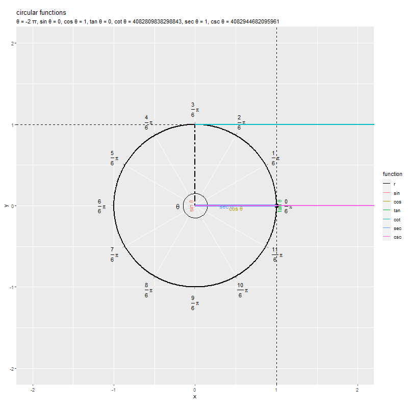
のとき
なので、原点と円周上の点を結ぶ線分が水平になり直線
と平行なため交点ができず、
を描画(定義)できないのが分かります。また、
のとき
なので、原点と円周上の点を結ぶ線分が垂直になり直線
と平行なため交点ができず、
を描画(定義)できないのが分かります。
パターン2
・作図コード(クリックで展開)
半径と円関数を示す線分の描画用のデータフレームを作成します。
# 関数直線の線分の座標を計算
anim_function_line_df <- tibble::tibble(
  fnc = c(
    "r", "r",
    "sin", "cos", "tan", "cot", "sec", "csc"
  ) |>
    rep(each = frame_num) |>
    factor(levels = fnc_level_vec), # 色用
  x_from = c(
    rep(0, times = frame_num), rep(0, times = frame_num),
    cos(theta_i),
    rep(0, times = frame_num),
    cos(theta_i),
    cos(theta_i),
    rep(0, times = frame_num),
    rep(0, times = frame_num)
  ),
  y_from = c(
    rep(0, times = frame_num), rep(0, times = frame_num),
    rep(0, times = frame_num),
    sin(theta_i),
    sin(theta_i),
    sin(theta_i),
    rep(0, times = frame_num),
    rep(0, times = frame_num)
  ),
  x_to = c(
    rep(1, times = frame_num), cos(theta_i),
    cos(theta_i),
    cos(theta_i),
    1/cos(theta_i),
    rep(0, times = frame_num),
    1/cos(theta_i),
    rep(0, times = frame_num)
  ),
  y_to = c(
    rep(0, times = frame_num), sin(theta_i),
    sin(theta_i),
    sin(theta_i),
    rep(0, times = frame_num),
    1/sin(theta_i),
    rep(0, times = frame_num),
    1/sin(theta_i)
  ),
  frame_label = frame_label_vec |>
    rep(times = 8) |> # (線分の数)
    factor(levels = frame_label_vec), # フレーム切替用ラベル
) |>
  dplyr::mutate(
    y_to = dplyr::if_else(condition = y_to == Inf, true = 1e+10, false = y_to)
  ) # 発散した場合は大きな値に置換
anim_function_line_df
## # A tibble: 1,440 × 6
##    fnc   x_from y_from  x_to  y_to frame_label
##    <fct>  <dbl>  <dbl> <dbl> <dbl> <fct>
##  1 r          0      0     1     0 θ = -2 π, sin θ = 0, cos θ = 1, tan θ =…
##  2 r          0      0     1     0 θ = -1.98 π, sin θ = 0.07, cos θ = 1, ta…
##  3 r          0      0     1     0 θ = -1.96 π, sin θ = 0.14, cos θ = 0.99,…
##  4 r          0      0     1     0 θ = -1.93 π, sin θ = 0.21, cos θ = 0.98,…
##  5 r          0      0     1     0 θ = -1.91 π, sin θ = 0.28, cos θ = 0.96,…
##  6 r          0      0     1     0 θ = -1.89 π, sin θ = 0.34, cos θ = 0.94,…
##  7 r          0      0     1     0 θ = -1.87 π, sin θ = 0.41, cos θ = 0.91,…
##  8 r          0      0     1     0 θ = -1.84 π, sin θ = 0.47, cos θ = 0.88,…
##  9 r          0      0     1     0 θ = -1.82 π, sin θ = 0.53, cos θ = 0.85,…
## 10 r          0      0     1     0 θ = -1.8 π, sin θ = 0.59, cos θ = 0.81, …
## # … with 1,430 more rows
「パターン1」のときと同様に、半径と関数の線分の座標を格納します。
関数名(ラベル)の描画用のデータフレームを作成します。
# 関数ラベルの座標を計算
anim_function_label_df <- anim_function_line_df |>
  dplyr::filter(fnc != "r") |> # 関数を抽出
  dplyr::group_by(fnc, frame_label) |> # 中点の計算用
  dplyr::summarise(
    x = median(c(x_from, x_to)),
    y = median(c(y_from, y_to)), .groups = "drop"
  ) |> # 線分の中点に配置
  tibble::add_column(
    angle = c(90, 0, 0, 0, 0, 90) |>
      rep(each = frame_num),
    h = c(0.5, 0.5, -0.2, -0.2, 0.5, 0.5) |>
      rep(each = frame_num),
    v = c(-0.5, -0.5, 0.5, 0.5, 1, 1) |>
      rep(each = frame_num),
    fnc_label = c("sin~theta", "cos~theta", "tan~theta", "cot~theta", "sec~theta", "csc~theta") |>
      rep(each = frame_num) # 関数ラベル
  )
anim_function_label_df
## # A tibble: 1,080 × 8
##    fnc   frame_label                   x        y angle     h     v fnc_label
##    <fct> <fct>                     <dbl>    <dbl> <dbl> <dbl> <dbl> <chr>
##  1 sin   θ = -2 π, sin θ = 0, cos… 1     1.22e-16    90   0.5  -0.5 sin~theta
##  2 sin   θ = -1.98 π, sin θ = 0.0… 0.998 3.49e- 2    90   0.5  -0.5 sin~theta
##  3 sin   θ = -1.96 π, sin θ = 0.1… 0.990 6.96e- 2    90   0.5  -0.5 sin~theta
##  4 sin   θ = -1.93 π, sin θ = 0.2… 0.978 1.04e- 1    90   0.5  -0.5 sin~theta
##  5 sin   θ = -1.91 π, sin θ = 0.2… 0.961 1.38e- 1    90   0.5  -0.5 sin~theta
##  6 sin   θ = -1.89 π, sin θ = 0.3… 0.940 1.71e- 1    90   0.5  -0.5 sin~theta
##  7 sin   θ = -1.87 π, sin θ = 0.4… 0.914 2.03e- 1    90   0.5  -0.5 sin~theta
##  8 sin   θ = -1.84 π, sin θ = 0.4… 0.883 2.35e- 1    90   0.5  -0.5 sin~theta
##  9 sin   θ = -1.82 π, sin θ = 0.5… 0.848 2.65e- 1    90   0.5  -0.5 sin~theta
## 10 sin   θ = -1.8 π, sin θ = 0.59… 0.809 2.94e- 1    90   0.5  -0.5 sin~theta
## # … with 1,070 more rows
関数ごとに1つの行(線分)を取り出して、それぞれ中点の座標を計算して、ラベル用の文字列などを格納します。
単位円上に円関数の線分を重ねたアニメーションを作成します。
# グラフサイズ用の値を指定
axis_size <- 2

# 単位円上の関数直線のアニメーションを作図
graphs <- ggplot() +
  geom_segment(data = radian_lable_df,
               mapping = aes(x = 0, y = 0, xend = x, yend = y),
               color = "white") + # 角度目盛グリッド
  geom_text(data = radian_lable_df,
            mapping = aes(x = x, y = y, angle = t_deg+90), label = "|",
            size = 2) + # 角度目盛指示線
  geom_text(data = radian_lable_df,
            mapping = aes(x = label_x, y = label_y, label = rad_label,
                          hjust = h, vjust = v), parse = TRUE) + # 角度目盛ラベル
  geom_path(data = anim_angle_mark_df,
            mapping = aes(x = x, y = y),
            size = 0.5) + # なす角マーク
  geom_text(data = anim_angle_label_df,
            mapping = aes(x = x, y = y), label = "theta", parse = TRUE,
            size = 5) + # なす角ラベル
  geom_path(data = circle_df,
            mapping = aes(x = x, y = y),
            size = 1) + # 円周
  geom_point(data = anim_point_df,
             mapping = aes(x = cos_t, y = sin_t),
             size = 4) + # 円周上の点
  geom_hline(yintercept = 0, linetype = "dashed") + # 補助線
  geom_vline(xintercept = 0, linetype = "dashed") + # 補助線
  geom_segment(data = anim_function_line_df,
               mapping = aes(x = x_from, y = y_from, xend = x_to, yend = y_to, color = fnc),
               size = 1) + # 関数直線
  geom_text(data = anim_function_label_df,
            mapping = aes(x = x, y = y, label = fnc_label, color = fnc,
                          hjust = h, vjust = v, angle = angle),
            parse = TRUE, show.legend = FALSE) + # 関数ラベル
  gganimate::transition_manual(frames = frame_label) + # フレーム
  scale_color_manual(breaks = fnc_level_vec,
                     values = c("black", scales::hue_pal()(length(fnc_level_vec)-1))) + # (半径直線を黒色にしたい)
  coord_fixed(ratio = 1,
              xlim = c(-axis_size, axis_size), ylim = c(-axis_size, axis_size)) + # 描画領域
  labs(title = "circular functions",
       subtitle = "{current_frame}",
       color = "function",
       x = "x", y = "y")

# gif画像を作成
anim <- gganimate::animate(plot = graphs, nframes = frame_num, fps = 100, width = 800, height = 800)
anim

こちらの図だと、 のとき、原点と円周上の点を結ぶ線分の垂線が垂直になり直線
と平行なため交点ができず、
を描画(定義)できないのが分かります。また、
のとき、原点と円周上の点を結ぶ線分の垂線が水平になり直線
と平行なため交点ができず、
を描画(定義)できないのが分かります。
なす角と関数曲線の関係
最後は、単位円上におけるなす角と円関数(sin・cos・tan・cot・sec・csc)の曲線の関係をグラフで可視化します。
グラフの作成
変数を固定した円関数をグラフで確認します。
・作図コード(クリックで展開)
変数の値を指定します。
# 単位円上の点用のラジアンを指定
theta <- 5/4 * pi
theta
## [1] 3.926991
単位円におけるなす角(ラジアン) を
thetaとして値を指定します。ただし、thetaが0のとき、計算結果にInfや-Infが含まれるため、意図しないグラフになります。発散時の対策については「アニメーションの作成」を参照してください。
「なす角と円関数の関係」の「パターン1」のコードで3つのデータフレーム(point_df・angle_mark_df・angle_label_df)を作成します。
半径と円関数を示す線分の描画用のデータフレームを作成します。
# 関数ラベルのレベルを指定
fnc_level_vec <- c("r", "sin", "cos", "tan", "cot", "sec", "csc")

# 反転フラグを設定
sin_flag <- sin(theta) >= 0
cos_flag <- cos(theta) >= 0

# 関数直線の線分の座標を計算
function_line_df <- tibble::tibble(
  fnc = c(
    "r", "r", "r", "r",
    "sin", "sin",
    "cos", "cos", "cos",
    "tan", "tan",
    "cot", "cot", "cot", "cot", "cot",
    "sec", "sec", "sec",
    "csc", "csc", "csc"
  ) |>
    factor(levels = fnc_level_vec), # 色用
  x_from = c(
    0, 0, 1/tan(theta), ifelse(test = cos_flag, yes = NA, no = -1/tan(theta)),
    0, cos(theta),
    0, 0, 0,
    1, ifelse(test = sin_flag, yes = NA, no = 1),
    0, 0, ifelse(test = cos_flag, yes = NA, no = 0), ifelse(test = cos_flag, yes = NA, no = 0), 0,
    0, ifelse(test = sin_flag, yes = NA, no = 0), 0,
    0, ifelse(test = cos_flag, yes = NA, no = 0), 0
  ),
  y_from = c(
    0, 0, 0, ifelse(test = cos_flag, yes = NA, no = 0),
    0, 0,
    0, sin(theta), 0,
    0, ifelse(test = sin_flag, yes = NA, no = 0),
    0, 1, ifelse(test = cos_flag, yes = NA, no = 0), ifelse(test = cos_flag, yes = NA, no = 1), 0,
    0, ifelse(test = sin_flag, yes = NA, no = 0), 0,
    0, ifelse(test = cos_flag, yes = NA, no = 0), 0
  ),
  x_to = c(
    1, cos(theta), 1/tan(theta), ifelse(test = cos_flag, yes = NA, no = -1/tan(theta)),
    0, cos(theta),
    cos(theta), cos(theta), 0,
    1, ifelse(test = sin_flag, yes = NA, no = 1),
    1/tan(theta), 1/tan(theta), ifelse(test = cos_flag, yes = NA, no = -1/tan(theta)), ifelse(test = cos_flag, yes = NA, no = -1/tan(theta)), 0,
    1, ifelse(test = sin_flag, yes = NA, no = 1), 0,
    ifelse(test = cos_flag, yes = 1/tan(theta), no = -1/tan(theta)), ifelse(test = cos_flag, yes = NA, no = 1/tan(theta)), 0
  ),
  y_to = c(
    0, sin(theta), 1, ifelse(test = cos_flag, yes = NA, no = 1),
    sin(theta), sin(theta),
    0, sin(theta), cos(theta),
    tan(theta), ifelse(test = sin_flag, yes = NA, no = -tan(theta)),
    0, 1, ifelse(test = cos_flag, yes = NA, no = 0), ifelse(test = cos_flag, yes = NA, no = 1), 1/tan(theta),
    ifelse(test = sin_flag, yes = tan(theta), no = -tan(theta)), ifelse(test = sin_flag, yes = NA, no = tan(theta)), 1/cos(theta),
    1, ifelse(test = cos_flag, yes = NA, no = 1), 1/sin(theta)
  ),
  width = c(
    "normal", "normal", "thin", "thin",
    "normal", "normal",
    "bold", "normal", "thin",
    "normal", "normal",
    "thin", "normal", "thin", "normal", "thin",
    "bold", "bold", "thin",
    "thin", "thin", "thin"
  ), # 太さ用
  type = c(
    "main", "main", "main", "main",
    "main", "main",
    "main", "main", "sub",
    "main", "sub",
    "main", "main", "sub", "sub", "sub",
    "main", "sub", "sub",
    "main", "sub", "sub"
    ), # 線種用
  label_flag = c(
    FALSE, FALSE, FALSE, FALSE,
    TRUE, FALSE,
    TRUE, FALSE, FALSE,
    TRUE, FALSE,
    TRUE, FALSE, FALSE, FALSE, FALSE,
    TRUE, FALSE, FALSE,
    TRUE, FALSE, FALSE
  ) # 関数ラベル用
)
function_line_df
## # A tibble: 22 × 8
##    fnc   x_from y_from   x_to   y_to width  type  label_flag
##    <fct>  <dbl>  <dbl>  <dbl>  <dbl> <chr>  <chr> <lgl>
##  1 r      0      0      1      0     normal main  FALSE
##  2 r      0      0     -0.707 -0.707 normal main  FALSE
##  3 r      1      0      1      1     thin   main  FALSE
##  4 r     -1      0     -1      1     thin   main  FALSE
##  5 sin    0      0      0     -0.707 normal main  TRUE
##  6 sin   -0.707  0     -0.707 -0.707 normal main  FALSE
##  7 cos    0      0     -0.707  0     bold   main  TRUE
##  8 cos    0     -0.707 -0.707 -0.707 normal main  FALSE
##  9 cos    0      0      0     -0.707 thin   sub   FALSE
## 10 tan    1      0      1      1     normal main  TRUE
## # … with 12 more rows
「なす角と円関数の関係」のときのコードに、cos・cot・sec・csc関数の線分の1つを垂直線に回転した線分の座標を追加します。
関数名(ラベル)の描画用のデータフレームを作成します。
# 関数ラベルの座標を計算
function_label_df <- function_line_df |>
  dplyr::filter(label_flag) |> # ラベル付けする線分を抽出
  dplyr::group_by(fnc) |> # 中点の計算用
  dplyr::summarise(
    x = median(c(x_from, x_to)),
    y = median(c(y_from, y_to)), .groups = "drop"
  ) |> # 線分の中点に配置
  tibble::add_column(
    angle = c(90, 0, 90, 0, 0, 0),
    h = c(0.5, 0.5, 0.5, 0.5, 1.2, -0.2),
    v = c(-0.5, 1, 1, -0.5, 0.5, 0.5),
    fnc_label = c("sin~theta", "cos~theta", "tan~theta", "cot~theta", "sec~theta", "csc~theta") # 関数ラベル
  )
function_label_df
## # A tibble: 6 × 7
##   fnc        x      y angle     h     v fnc_label
##   <fct>  <dbl>  <dbl> <dbl> <dbl> <dbl> <chr>
## 1 sin    0     -0.354    90   0.5  -0.5 sin~theta
## 2 cos   -0.354  0         0   0.5   1   cos~theta
## 3 tan    1      0.5      90   0.5   1   tan~theta
## 4 cot    0.5    0         0   0.5  -0.5 cot~theta
## 5 sec    0.5   -0.5       0   1.2   0.5 sec~theta
## 6 csc   -0.5    0.5       0  -0.2   0.5 csc~theta
関数ごとに1つの行(線分)を取り出して、それぞれ中点の座標を計算して、ラベル用の文字列などを格納します。
関数直線を垂直線になるように回転する軌道の描画用のデータフレームを作成します。
# sec・csc直線の角度を設定
if(cos(theta) >= 0) {
  theta_sec <- acos(cos(theta))
} else {
  theta_sec <- pi + acos(cos(theta))
}
if(sin(theta) >= 0) {
  theta_csc <- asin(sin(theta))
} else {
  theta_csc <- pi + asin(sin(theta))
}

# 軸変換曲線の座標を計算
num <- 100
adapt_curve_df <- tibble::tibble(
  fnc = c(
    rep("cos", times = num),
    rep("cot", times = num),
    rep("sec", times = num),
    rep("csc", times = num)
  ), # 色用
  rad = c(
    seq(from = 0, to = 0.5*pi, length.out = num),
    seq(from = 0, to = 0.5*pi, length.out = num),
    seq(from = theta_sec, to = ifelse(test = cos(theta) >= 0, yes = 0.5*pi, no = 1.5*pi), length.out = num),
    seq(from = theta_csc, to = ifelse(test = sin(theta) >= 0, yes = 0.5*pi, no = 1.5*pi), length.out = num)
  ),
  d = c(
    rep(cos(theta), times = num),
    rep(1/tan(theta), times = num),
    rep(abs(1/cos(theta)), times = num),
    rep(abs(1/sin(theta)), times = num)
  ),
  x = d * cos(rad),
  y = d * sin(rad)
)
adapt_curve_df
## # A tibble: 400 × 5
##    fnc      rad      d      x       y
##    <chr>  <dbl>  <dbl>  <dbl>   <dbl>
##  1 cos   0      -0.707 -0.707  0
##  2 cos   0.0159 -0.707 -0.707 -0.0112
##  3 cos   0.0317 -0.707 -0.707 -0.0224
##  4 cos   0.0476 -0.707 -0.706 -0.0336
##  5 cos   0.0635 -0.707 -0.706 -0.0448
##  6 cos   0.0793 -0.707 -0.705 -0.0560
##  7 cos   0.0952 -0.707 -0.704 -0.0672
##  8 cos   0.111  -0.707 -0.703 -0.0784
##  9 cos   0.127  -0.707 -0.701 -0.0895
## 10 cos   0.143  -0.707 -0.700 -0.101
## # … with 390 more rows
軸を変換する軌道として、半径が各関数の絶対値 の円弧を描画します。全体値
は
abs()で計算できます。詳しくはそれぞれの関数の記事を参照してください。
単位円における点と関数曲線上の点を結ぶ補助線(の一部)の描画用のデータフレームを作成します。
# グラフサイズ用の値を設定
axis_lower <- 1.5
axis_upper <- 4
x_size <- c(1/sin(theta), 1/tan(theta)) |> # csc・cot
  abs() |> # 絶対値
  ceiling() |> # 切り上げ
  max(axis_lower) |> # 下限
  min(axis_upper) # 上限
y_size <- c(1/cos(theta), 1/sin(theta), 1/tan(theta)) |> # sec・csc・cot
  abs() |> # 絶対値
  ceiling() |> # 切り上げ
  max(axis_lower) |> # 下限
  min(axis_upper) # 上限

# 関数曲線との対応線の座標を計算
l <- 0.5
segment_circle_df <- tibble::tibble(
  fnc = c("sin", "cos", "tan", "sec", "csc", "cot") |>
    factor(levels = fnc_level_vec), # 色用
  #x = c(0, 0, 0, 0, 0, 0), # y軸線上に並べる場合
  x = c(cos(theta), 0, 1, 0, 0, 0),
  y = c(sin(theta), cos(theta), tan(theta), 1/cos(theta), 1/sin(theta), 1/tan(theta)),
  x_to = x_size+l,
  y_to = y
)
segment_circle_df
## # A tibble: 6 × 5
##   fnc        x      y  x_to   y_to
##   <fct>  <dbl>  <dbl> <dbl>  <dbl>
## 1 sin   -0.707 -0.707   2.5 -0.707
## 2 cos    0     -0.707   2.5 -0.707
## 3 tan    1      1       2.5  1
## 4 sec    0     -1.41    2.5 -1.41
## 5 csc    0     -1.41    2.5 -1.41
## 6 cot    0      1       2.5  1
単位円図における点からy軸線の反対側へ水平線を引くように線分の座標を指定します。
単位円上に円関数の線分を重ねたグラフを作成します。
# 変数ラベル用の文字列を作成
variable_label <- paste0(
  "list(",
  "theta==", round(theta/pi, digits = 2), "*pi",
  ", sin~theta==", round(sin(theta), digits = 2),
  ", cos~theta==", round(cos(theta), digits = 2),
  ")"
)

# 単位円上に関数直線を作図
circle_graph <- ggplot() +
  geom_segment(data = radian_lable_df,
               mapping = aes(x = 0, y = 0, xend = x, yend = y),
               color = "white") + # 角度目盛グリッド
  geom_text(data = radian_lable_df,
            mapping = aes(x = x, y = y, angle = t_deg+90), label = "|",
            size = 2) + # 角度目盛指示線
  geom_text(data = radian_lable_df,
            mapping = aes(x = label_x, y = label_y, label = rad_label,
                          hjust = h, vjust = v), parse = TRUE) + # 角度目盛ラベル
  geom_path(data = angle_mark_df,
            mapping = aes(x = x, y = y),
            size = 0.5) + # なす角マーク
  geom_text(data = angle_label_df,
            mapping = aes(x = x, y = y), label = "theta", parse = TRUE,
            size = 5) + # なす角ラベル
  geom_path(data = circle_df,
            mapping = aes(x = x, y = y),
            size = 1) + # 円周
  geom_point(data = point_df,
             mapping = aes(x = cos_t, y = sin_t),
             size = 4) + # 円周上の点
  geom_hline(yintercept = 1, linetype = "dashed") + # 補助線
  geom_vline(xintercept = 1, linetype = "dashed") + # 補助線
  geom_segment(data = function_line_df,
               mapping = aes(x = x_from, y = y_from, xend = x_to, yend = y_to,
                             color = fnc, size = width, linetype = type), na.rm = TRUE) + # 関数直線
  geom_text(data = function_label_df,
            mapping = aes(x = x, y = y, label = fnc_label, color = fnc,
                          hjust = h, vjust = v, angle = angle),
            parse = TRUE, na.rm = TRUE, show.legend = FALSE) + # 関数ラベル
  geom_path(data = adapt_curve_df,
            mapping = aes(x = x, y = y, color = fnc),
            size = 1, linetype = "dotted", show.legend = FALSE) + # 変換曲線
  geom_point(data = segment_circle_df,
             mapping = aes(x = x, y = y, color = fnc),
             size = 4, alpha = 0.5) + # 変換点
  geom_segment(data = segment_circle_df,
               mapping = aes(x = x, y = y, xend = x_to, yend = y, color = fnc),
               size = 1, linetype = "dotted", show.legend = FALSE) + # 関数曲線との対応線
  scale_color_manual(breaks = fnc_level_vec,
                     values = c("black", scales::hue_pal()(length(fnc_level_vec)-1))) + # (半径直線を黒色にしたい)
  scale_size_manual(breaks = c("normal", "bold", "thin"),
                    values = c(1, 1.6, 0.8), guide = "none") + # (線が重なる対策)
  scale_linetype_manual(breaks = c("main", "sub"),
                        values = c("solid", "twodash"), guide = "none") + # (補助線を描き分けたい)
  coord_fixed(ratio = 1, clip = "off",
              xlim = c(-x_size, x_size), ylim = c(-y_size, y_size)) + # 描画領域
  labs(title = "circular functions",
       subtitle = parse(text = variable_label),
       color = "function",
       x = "x", y = "y")
circle_graph

「なす角と円関数の関係」のときと同様に、単位円と関数直線を描画します。
関数曲線の描画用のデータフレームを作成します。
# 関数曲線用のラジアンを指定
theta_vec <- seq(from = 0, to = 2*pi, length.out = 1000)

# 円関数を計算
function_curve_df <- tibble::tibble(
  fnc = c("sin", "cos", "tan", "cot", "sec", "csc") |>
    rep(each = length(theta_vec)) |>
    factor(levels = fnc_level_vec), # 色用
  t = theta_vec |>
    rep(times = 6), # (関数の数)
  f_t = c(
    sin(theta_vec),
    cos(theta_vec),
    tan(theta_vec),
    1/tan(theta_vec),
    1/cos(theta_vec),
    1/sin(theta_vec)
  )
) |>
  dplyr::mutate(
    f_t = dplyr::if_else(
      (f_t >= -y_size & f_t <= y_size), true = f_t, false = NA_real_
    ) # 閾値外の値を欠損値に置換
  )
function_curve_df
## # A tibble: 6,000 × 3
##    fnc         t     f_t
##    <fct>   <dbl>   <dbl>
##  1 sin   0       0
##  2 sin   0.00629 0.00629
##  3 sin   0.0126  0.0126
##  4 sin   0.0189  0.0189
##  5 sin   0.0252  0.0252
##  6 sin   0.0314  0.0314
##  7 sin   0.0377  0.0377
##  8 sin   0.0440  0.0440
##  9 sin   0.0503  0.0503
## 10 sin   0.0566  0.0566
## # … with 5,990 more rows
「円関数の作図」のときと同様に、各円関数を計算します。
関数曲線上の点と単位円における点を結ぶ補助線(の一部)の描画用のデータフレームを作成します。
# 関数直線との対応線の座標を計算
l <- 0.7
segment_curve_df <- tibble::tibble(
  fnc = c("sin", "cos", "tan", "cot", "sec", "csc") |>
    factor(levels = fnc_level_vec),
  x = theta,
  y = c(sin(theta), cos(theta), tan(theta), 1/tan(theta), 1/cos(theta), 1/sin(theta)),
  x_to = -l,
  y_to = y
)
segment_curve_df
## # A tibble: 6 × 5
##   fnc       x      y  x_to   y_to
##   <fct> <dbl>  <dbl> <dbl>  <dbl>
## 1 sin    3.93 -0.707  -0.7 -0.707
## 2 cos    3.93 -0.707  -0.7 -0.707
## 3 tan    3.93  1      -0.7  1
## 4 cot    3.93  1      -0.7  1
## 5 sec    3.93 -1.41   -0.7 -1.41
## 6 csc    3.93 -1.41   -0.7 -1.41
曲線上の点からy軸線へ水平線を引くように線分の座標を指定します。
x軸目盛の設定用のベクトルを作成します。
# 半周期の目盛の数(分母の値)を指定
denom <- 6

# 目盛の通し番号(分子の値)を作成
numer_vec <- seq(from = 0, to = 2*pi / pi * denom, by = 1)

# 目盛ラベル用の文字列を作成
label_vec <- paste0(c("", "-")[(numer_vec < 0)+1], "frac(", abs(numer_vec), ", ", denom, ")~pi")
head(numer_vec); head(label_vec)
## [1] 0 1 2 3 4 5
## [1] "frac(0, 6)~pi" "frac(1, 6)~pi" "frac(2, 6)~pi" "frac(3, 6)~pi"
## [5] "frac(4, 6)~pi" "frac(5, 6)~pi"
「円関数の作図」のときと同様にして、目盛ラベル用の値と文字列を作成します。
関数曲線のグラフを作成します。
# 変数ラベル用の文字列を作成
variable_label <- paste0(
  "list(",
  "theta==", round(theta, digits = 2),
  ", sin~theta==", round(sin(theta), digits = 2),
  ", cos~theta==", round(cos(theta), digits = 2),
  ", tan~theta==", round(tan(theta), digits = 2),
  ", cot~theta==", round(1/tan(theta), digits = 2),
  ", sec~theta==", round(1/cos(theta), digits = 2),
  ", csc~theta==", round(1/sin(theta), digits = 2),
  ")"
)

# 関数曲線を作図
curve_graph <- ggplot() +
  geom_vline(xintercept = theta, linetype = "dashed") + # 変数垂線
  geom_line(data = function_curve_df,
            mapping = aes(x = t, y = f_t, color = fnc), na.rm = TRUE,
            size = 1) + # 関数曲線
  geom_point(data = segment_curve_df,
             mapping = aes(x = x, y = y, color = fnc),
             size = 4, alpha = 0.5) + # 曲線上の点
  geom_segment(data = segment_curve_df,
               mapping = aes(x = x, y = y, xend = x_to, yend = y, color = fnc),
               size = 1, linetype = "dotted") + # 関数直線との対応線
  scale_x_continuous(breaks = numer_vec/denom*pi,
                     labels = parse(text = label_vec)) + # 角度目盛ラベル
  coord_fixed(ratio = 1, clip = "off",
              xlim = c(0, 2*pi), ylim = c(-y_size, y_size)) + # 描画領域
  theme(legend.position = "none") + # 図の体裁
  labs(title = "",
       subtitle = parse(text = variable_label),
       x = expression(theta),
       y = expression(f(theta)))
curve_graph

「円関数の作図」のときと同様に、関数曲線を描画します。
2つのグラフを並べて描画します。
# 並べて描画
graph <- patchwork::wrap_plots(circle_graph, curve_graph, guides = "collect")
graph
patchworkパッケージのwrap_plots()を使ってグラフを並べます。

2つのグラフで、単位円図における各関数を表す線分の「長さと座標の正負」と曲線上の点の「y軸の値」が対応するのが分かります。また、なす角の値とx軸の値が一致します。
アニメーションの作成
続いて、変数の値を変化させた円関数をアニメーションで確認します。詳しくはGitHubを参照してください。
1周
円周上を1周した際の円関数の線分と曲線上の点の関係を可視化します。

となる
とき、cot関数とcsc関数の線分の象限(
の符号)が変わり、cot関数とcsc関数の曲線が不連続になるのが分かります。また、
となる
とき、tan関数とsec関数の線分の象限(
の符号)が変わり、tan関数とsec関数の曲線が不連続になるのが分かります。
n周
円周上を複数回周回した際の円関数の線分と曲線上の点の関係を可視化します。

単位円上の点が1周する (tan関数の場合は半周する
)の間隔で、それぞれの関数の曲線が同じ形になるのが分かります。
この記事では、6つの円関数を可視化しました。
おわりに
新年一発目の記事です。今年は数学力を鍛えたい。ということで、とりあえず三角関数からやっていきます。
2023年1月7日は、モーニング娘。'23の石田亜佑美さんの26歳のお誕生日です。
26歳!おめでとうございます。あゆみんリーダー体制を待ってます!(2023年ってことにびっくりする。)
(追記:公開終了していますがこのままにしておきます。ハロプロダンス学園とDA PUMPのKENZOのコラボ企画のダンス動画でした。)
- 2023.07.09:加筆修正しました。
よく目にする3つの関数sin・cos・tanの可視化だった内容に、csc・sec・cotを加えて可視化のバリエーションも増やしました。また、この記事で全ての関数を簡単に比較して個別の記事でそれぞれ深掘りする構成だったのを、個別の記事で確認してからこの記事で比較するように再構成しました。
ここまで来るのに半年かかりました。このまとめ記事を書いてたらここまでのコードや内容を書き直したくなったのですが、やっぱり暫く触りたくない気もします。
何の役に立つのか分はからないままですが、自分なりに理解できたので良かったです。
最後に一番伝えたいことは「三角関数じゃなくて円関数って呼ぼうよっ!」です。よろしくお願いします。
大団円!
【他の記事一覧】