はじめに
円関数(三角関数)の定義や性質、公式などを可視化して理解しようシリーズです。
この記事では、R言語でcosecant関数のグラフを作成します。
【前の内容】
【他の記事一覧】
【この記事の内容】
csc関数の定義の可視化
csc関数(余割関数・コセカント関数・cosecant function)の定義をグラフで確認します。csc関数は、円関数(circular functions)・三角関数(trigonometric functions)の1つです。
csc関数の形状(振幅・周期・位相・切片)の変化については各パラメータの記事や「csc関数の波形の可視化」を参照してください。
利用するパッケージを読み込みます。
# 利用パッケージ
library(tidyverse)
この記事では、基本的に パッケージ名::関数名() の記法を使うので、パッケージの読み込みは不要です。ただし、作図コードについてはパッケージ名を省略するので、ggplot2 を読み込む必要があります。
また、ネイティブパイプ演算子 |> を使います。magrittr パッケージのパイプ演算子 %>% に置き換えられますが、その場合は magrittr を読み込む必要があります。
定義式の確認
まずは、csc関数の定義式を確認します。
sin関数については「【R】sin関数の定義の可視化 - からっぽのしょこ」を参照してください。
csc関数は、sin関数の逆数で定義されます。
ただし、 を正負の整数として
のとき、
であり、0除算になるため定義できません。変数
はラジアン(弧度法の角度)、
は円周率です。
曲線の形状
続いて、csc関数の曲線のグラフを作成します。
曲線の作成
・作図コード(クリックで展開)
変数の範囲を指定して、座標計算用のベクトルを作成します。
# 変数(ラジアン)の範囲を指定
theta_vec <- seq(from = -2*pi, to = 2*pi, length.out = 1001)
head(theta_vec)
[1] -6.283185 -6.270619 -6.258053 -6.245486 -6.232920 -6.220353
変数(ラジアン) の範囲を指定して、数値ベクトルを作成します。範囲を
の倍数にすると周期性を確認しやすくなります。円周率
は
pi で扱えます。
曲線の描画用のデータフレームを作成します。
# 閾値を指定
threshold <- 4

# 曲線の座標を作成
curve_df <- tibble::tibble(
  t     = theta_vec,
  csc_t = 1/sin(t),
  sin_t = sin(t),
  sec_t = 1/cos(t)
) |>
  dplyr::mutate(
    csc_t = dplyr::if_else(
      (csc_t >= -threshold & csc_t <= threshold), true = csc_t, false = NA_real_
    ),
    sec_t = dplyr::if_else(
      (sec_t >= -threshold & sec_t <= threshold), true = sec_t, false = NA_real_
    )
  ) # 閾値外を欠損値に置換
curve_df
# A tibble: 1,001 × 4
       t csc_t    sin_t sec_t
   <dbl> <dbl>    <dbl> <dbl>
 1 -6.28    NA 2.45e-16  1
 2 -6.27    NA 1.26e- 2  1.00
 3 -6.26    NA 2.51e- 2  1.00
 4 -6.25    NA 3.77e- 2  1.00
 5 -6.23    NA 5.02e- 2  1.00
 6 -6.22    NA 6.28e- 2  1.00
 7 -6.21    NA 7.53e- 2  1.00
 8 -6.20    NA 8.79e- 2  1.00
 9 -6.18    NA 1.00e- 1  1.01
10 -6.17    NA 1.13e- 1  1.01
# ℹ 991 more rows
変数 と関数
の値をデータフレームに格納します。比較用に、
の値も格納しておきます。sin関数は
sin() で、csc関数は sin()、sec関数は cos() を使って計算できます。
ただし範囲によっては、 が発散するので、閾値
threshold を指定しておき、閾値外の値を(数値型の)欠損値 NA に置き換えます。
ラジアン軸目盛の表示用のベクトルを作成します。装飾用の処理です。
# 半周期(範囲π)における目盛数(分母の値)を指定
tick_num <- 2

# 目盛番号(分子の値)の範囲を設定
tick_min <- floor(min(theta_vec) / pi) * tick_num
tick_max <- ceiling(max(theta_vec) / pi) * tick_num

# 目盛番号(分子の値)を作成
tick_vec <- tick_min:tick_max

# 目盛位置を作成
rad_break_vec <- tick_vec/tick_num * pi

# 目盛ラベルを作成
rad_label_vec <- paste(round(rad_break_vec/pi, digits = 2), "* pi")
head(tick_vec); head(rad_break_vec); head(rad_label_vec)
[1] -4 -3 -2 -1  0  1
[1] -6.283185 -4.712389 -3.141593 -1.570796  0.000000  1.570796
[1] "-2 * pi"   "-1.5 * pi" "-1 * pi"   "-0.5 * pi" "0 * pi"    "0.5 * pi"
ラジアン に関する軸目盛ラベルを
を小数にした形で表示することにします。
は半周期(
間隔の範囲)における目盛数、
は(負の数を含む)目盛番号に対応します。
theta_vec の最小値・最大値に対して、 を
について整理した
を計算して、最小番号から最大番号までの整数を作成します。整数にするために、小数部分に関して最小値は
floor() で切り捨て、最大値は ceiling() で切り上げておきます。
作成した目盛番号に対応する目盛位置(ラジアン)を で計算します。
ラベルとして数式(ギリシャ文字や記号)を表示する場合は、expression() の記法を用います。その際に、オブジェクト(プログラム上の変数)を使う場合は、文字列として作成しておき parse() の text 引数に渡します。
漸近線の描画用のベクトルを作成します。
# 漸近線の範囲を設定:(π単位で切り捨て・切り上げ)
theta_lower <- floor(min(theta_vec) / pi) * pi
theta_upper <- ceiling(max(theta_vec) / pi) * pi

# 漸近線の位置を作成
asymptote_break_vec <- seq(from = theta_lower, to = theta_upper, by = pi)

# 漸近線のラベルを作成
asymptote_label_vec <- paste(round(asymptote_break_vec/pi, digits = 2), "* pi")
head(asymptote_break_vec); head(asymptote_label_vec)
[1] -6.283185 -3.141593  0.000000  3.141593  6.283185
[1] "-2 * pi" "-1 * pi" "0 * pi"  "1 * pi"  "2 * pi"
が発散する位置に漸近線と目盛ラベルを表示することにします。
ラジアン軸目盛と同様に、theta_vec の最小値・最大値を用いて、ラジアン (
は整数)とラベルを作成します。
csc関数(とsin関数)のグラフを作成します。
# 関数曲線を作図
ggplot() +
  geom_segment(mapping = aes(x = c(-Inf, 0), y = c(0, -Inf),
                             xend = c(Inf, 0), yend = c(0, Inf)),
               arrow = arrow(length = unit(10, units = "pt"), ends = "last")) + # x・y軸線
  geom_vline(xintercept = asymptote_break_vec,
             linetype = "twodash") + # 漸近線
  geom_line(data = curve_df,
            mapping = aes(x = t, y = csc_t, linetype = "csc"),
            linewidth = 1, na.rm = TRUE) + # csc曲線
  geom_line(data = curve_df,
            mapping = aes(x = t, y = sin_t, linetype = "sin"),
            linewidth = 1) + # sin曲線
  scale_linetype_manual(breaks = c("csc", "sin"),
                        values = c("solid", "dotted"),
                        labels = c(expression(csc~theta), expression(sin~theta)),
                        name = "function") + # 凡例表示用
  scale_x_continuous(breaks = rad_break_vec,
                     labels = parse(text = rad_label_vec),
                     sec.axis = sec_axis(trans = ~.,
                                         breaks = asymptote_break_vec,
                                         labels = parse(text = asymptote_label_vec),
                                         name = "asymptote")) + # ラジアン軸目盛
  guides(linetype = guide_legend(override.aes = list(linewidth = 0.5))) + # 凡例の体裁
  theme(legend.text.align = 1) + # 図の体裁
  coord_fixed(ratio = 1) + # アスペクト比
  labs(title = "cosecant function",
       subtitle = expression(csc~theta == frac(1, sin~theta)),
       x = expression(theta),
       y = expression(f(theta)))
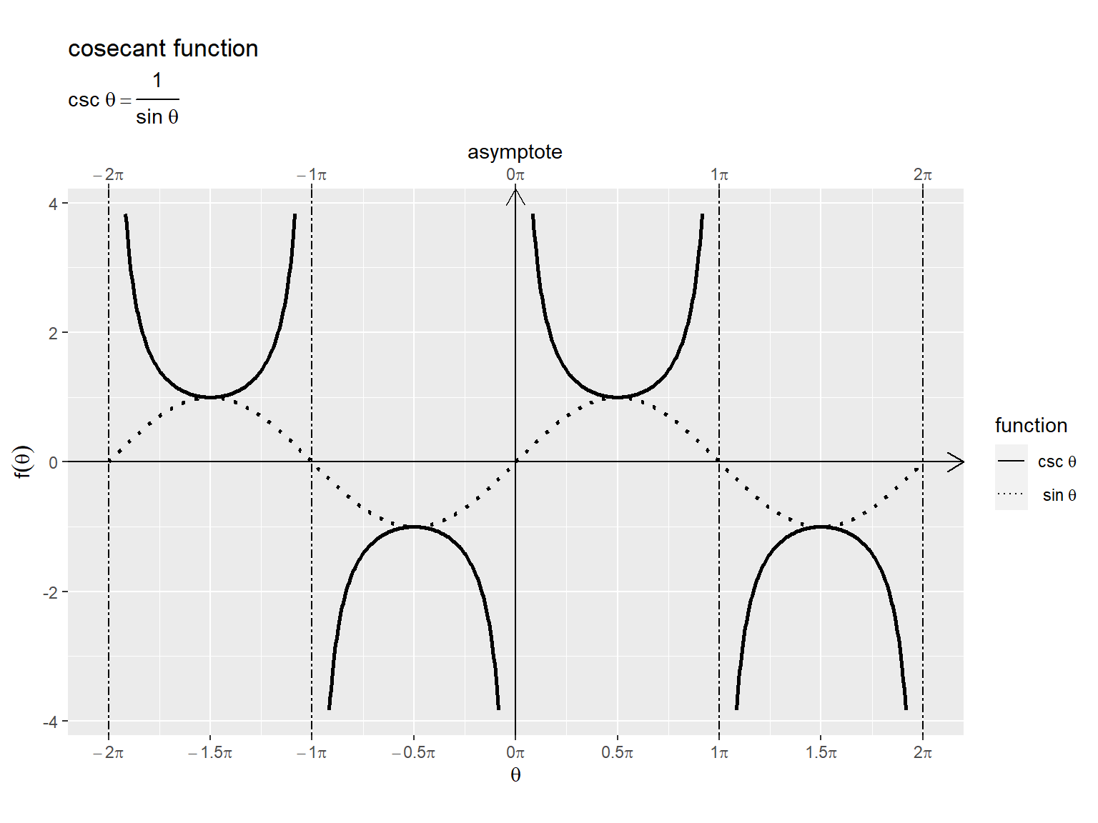
csc曲線を実線、sin曲線を点線で、また漸近線を鎖線で示します。
横軸(変数) はラジアン(弧度法の角度)、
は円周率です。
を整数として、
軸が
の点(
を中心に
間隔)で、
であり、
が発散するのを確認できます。
・作図コード(クリックで展開)
csc関数(とsec関数)のグラフを作成します。
# 関数曲線を作図
ggplot() +
  geom_segment(mapping = aes(x = c(-Inf, 0), y = c(0, -Inf),
                             xend = c(Inf, 0), yend = c(0, Inf)),
               arrow = arrow(length = unit(10, units = "pt"), ends = "last")) + # x・y軸線
  geom_vline(xintercept = asymptote_break_vec,
             linetype = "twodash") + # 漸近線
  geom_line(data = curve_df,
            mapping = aes(x = t, y = csc_t, linetype = "csc"),
            linewidth = 1, na.rm = TRUE) + # csc曲線
  geom_line(data = curve_df,
            mapping = aes(x = t, y = sec_t, linetype = "sec"),
            linewidth = 1) + # sec曲線
  scale_linetype_manual(breaks = c("csc", "sec"),
                        values = c("solid", "dotted"),
                        labels = c(expression(csc~theta), expression(sec~theta)),
                        name = "function") + # 凡例表示用
  scale_x_continuous(breaks = rad_break_vec,
                     labels = parse(text = rad_label_vec),
                     sec.axis = sec_axis(trans = ~.,
                                         breaks = asymptote_break_vec,
                                         labels = parse(text = asymptote_label_vec),
                                         name = "asymptote")) + # ラジアン軸目盛
  guides(linetype = guide_legend(override.aes = list(linewidth = 0.5))) + # 凡例の体裁
  theme(legend.text.align = 1) + # 図の体裁
  coord_fixed(ratio = 1) + # アスペクト比
  labs(title = "cosecant function",
       subtitle = expression(csc~theta == frac(1, sin~theta)),
       x = expression(theta),
       y = expression(f(theta)))
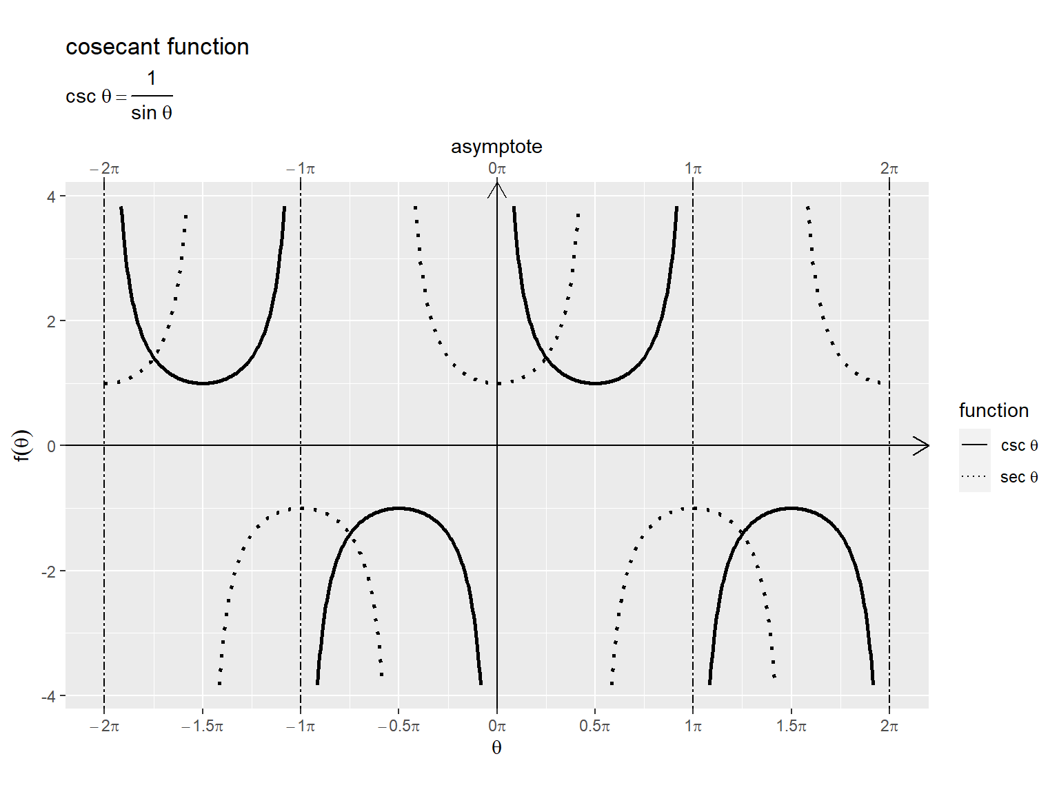
csc曲線を実線、sec曲線を点線で示します。
余角の関係より、 が成り立ちます。
次からは、単位円との関係を見ていきます。
単位円の作成
円関数の可視化に利用する単位円(unit circle)のグラフを確認します。
円の作図や度数法と弧度法(角度とラジアン)の関係については「【R】円周の作図 - からっぽのしょこ」を参照してください。
・作図コード(クリックで展開)
単位円の描画用のデータフレームを作成します。
# 円周の座標を作成
circle_df <- tibble::tibble(
  t = seq(from = 0, to = 2*pi, length.out = 361), # 1周期分のラジアン
  r = 1, # 半径
  x = r * cos(t),
  y = r * sin(t)
)
circle_df
# A tibble: 361 × 4
        t     r     x      y
    <dbl> <dbl> <dbl>  <dbl>
 1 0          1 1     0
 2 0.0175     1 1.00  0.0175
 3 0.0349     1 0.999 0.0349
 4 0.0524     1 0.999 0.0523
 5 0.0698     1 0.998 0.0698
 6 0.0873     1 0.996 0.0872
 7 0.105      1 0.995 0.105
 8 0.122      1 0.993 0.122
 9 0.140      1 0.990 0.139
10 0.157      1 0.988 0.156
# ℹ 351 more rows
1周分のラジアン を作成して、単位円の円周のx座標
とy座標
を計算します。
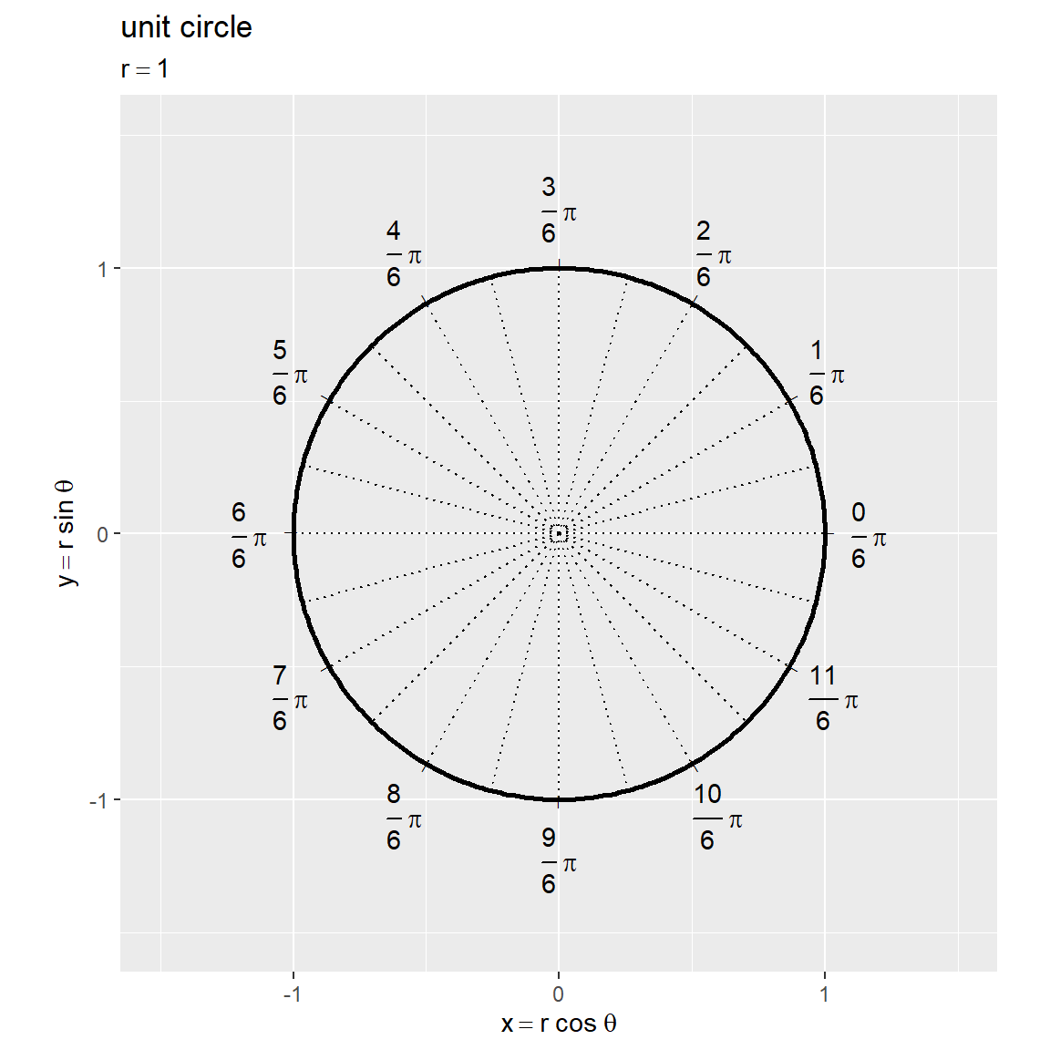
角度(ラジアン)目盛の描画用のデータフレームを作成します。
# 半円(範囲π)における目盛数(分母の値)を指定
tick_num <- 6

# 角度目盛の座標を作成:(補助目盛有り)
d <- 1.1
rad_tick_df <- tibble::tibble(
  # 座標用
  i     = seq(from = 0, to = 2*tick_num-0.5, by = 0.5), # 目盛番号(分子の値)
  t_deg = i/tick_num * 180, # 度数法の角度
  t_rad = i/tick_num * pi,  # 弧度法の角度(ラジアン)
  r     = 1, # 半径
  x     = r * cos(t_rad),
  y     = r * sin(t_rad),
  major_flag = i%%1 == 0, # 主・補助フラグ
  grid       = dplyr::if_else(major_flag, true = "major", false = "minor"), # 目盛カテゴリ
  # ラベル用
  deg_label  = dplyr::if_else(
    major_flag, true = paste0(round(t_deg, digits = 1), "*degree"), false = ""
  ), # 角度ラベル
  rad_label  = dplyr::if_else(
    major_flag, true = paste0("frac(", i, ", ", tick_num, ") ~ pi"), false = ""
  ), # ラジアンラベル
  label_x = d * x,
  label_y = d * y,
  a = t_deg + 90,
  h = 1 - (x * 0.5 + 0.5),
  v = 1 - (y * 0.5 + 0.5),
  tick_mark = dplyr::if_else(major_flag, true = "|", false = "") # 目盛指示線用
)
rad_tick_df
# A tibble: 24 × 16
       i t_deg t_rad     r         x     y major_flag grid  deg_label  rad_label
   <dbl> <dbl> <dbl> <dbl>     <dbl> <dbl> <lgl>      <chr> <chr>      <chr>
 1   0       0 0         1  1   e+ 0 0     TRUE       major "0*degree" "frac(0,…
 2   0.5    15 0.262     1  9.66e- 1 0.259 FALSE      minor ""         ""
 3   1      30 0.524     1  8.66e- 1 0.5   TRUE       major "30*degre… "frac(1,…
 4   1.5    45 0.785     1  7.07e- 1 0.707 FALSE      minor ""         ""
 5   2      60 1.05      1  5   e- 1 0.866 TRUE       major "60*degre… "frac(2,…
 6   2.5    75 1.31      1  2.59e- 1 0.966 FALSE      minor ""         ""
 7   3      90 1.57      1  6.12e-17 1     TRUE       major "90*degre… "frac(3,…
 8   3.5   105 1.83      1 -2.59e- 1 0.966 FALSE      minor ""         ""
 9   4     120 2.09      1 -5   e- 1 0.866 TRUE       major "120*degr… "frac(4,…
10   4.5   135 2.36      1 -7.07e- 1 0.707 FALSE      minor ""         ""
# ℹ 14 more rows
# ℹ 6 more variables: label_x <dbl>, label_y <dbl>, a <dbl>, h <dbl>, v <dbl>,
#   tick_mark <chr>
「曲線の作図」のときと同様に、目盛番号と対応するラジアンを作成して、円周上の座標とラベル用の文字列を作成します。ただし、補助目盛も作成します。主目盛と補助目盛を major_flag 列または grid 列で描き分けます。
目盛ラベル用の座標を label_x, label_y 列として、表示位置を原点からのノルム(半径) d で調整します。
単位円と角度目盛のグラフを作成します。
# グラフサイズを設定
axis_size <- 1.5

# 単位円を作図
ggplot() +
  geom_segment(data = rad_tick_df,
               mapping = aes(x = 0, y = 0, xend = x, yend = y),
               linetype = "dotted") + # 角度目盛線
  geom_text(data = rad_tick_df,
            mapping = aes(x = x, y = y, angle = a, label = tick_mark),
            size = 2) + # 角度目盛指示線
  geom_text(data = rad_tick_df,
            mapping = aes(x = label_x, y = label_y, label = deg_label, hjust = h, vjust = v),
            parse = TRUE) + # 角度目盛ラベル
  geom_path(data = circle_df,
            mapping = aes(x = x, y = y),
            linewidth = 1) + # 円周
  coord_fixed(ratio = 1,
              xlim = c(-axis_size, axis_size),
              ylim = c(-axis_size, axis_size)) + # アスペクト比
  labs(title = "unit circle",
       subtitle = expression(r == 1),
       x = expression(x == r ~ cos~theta),
       y = expression(y == r ~ sin~theta))
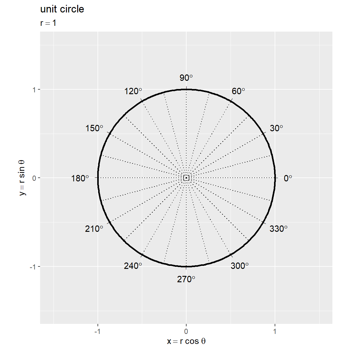
原点を中心とする半径 の円周の座標は
です。半径が
の円を単位円と呼びます。(半径や開始位置に関わらず)偏角が
(度数法だと
)で1周します。
度数法の角度 と弧度法の角度
は
の関係です。
このグラフ上に円関数の値を線分として描画します。
単位円と関数の関係
次は、単位円における偏角(単位円周上の点)と円関数(csc・sin・cos・cot)の関係を可視化します。
各関数についてはそれぞれの記事を参照してください。
グラフの作成
変数を固定して、単位円におけるcsc関数のグラフを作成します。
・作図コード(クリックで展開)
変数を指定して、円周上の点の描画用のデータフレームを作成します。
# 点用のラジアンを指定
theta <- 5/6 * pi

# 円周上の点の座標を作成
point_df <- tibble::tibble(
  t = theta,
  x = cos(t),
  y = sin(t)
)
point_df
# A tibble: 1 × 3
      t      x     y
  <dbl>  <dbl> <dbl>
1  2.62 -0.866   0.5
変数 を指定して、単位円の円周上の点の座標
を計算します。
の場合、
なので
1/sin(theta) が Inf になります。 以外(
など)の場合はプログラム上の誤差のため
sin(theta) が 0 になりません。ggplot2による作図では、Inf は描画領域の端を表すため意図しないグラフになることがあります。変数に微小な値を加えるなどして回避できます。
角マークの描画用のデータフレームを作成します。
# 角マークの座標を作成
d  <- 0.2
ds <- 0.005
angle_mark_df <- tibble::tibble(
  u = seq(from = 0, to = theta, length.out = 600),
  x = (d + ds*u) * cos(u),
  y = (d + ds*u) * sin(u)
)
angle_mark_df
# A tibble: 600 × 3
         u     x        y
     <dbl> <dbl>    <dbl>
 1 0       0.2   0
 2 0.00437 0.200 0.000874
 3 0.00874 0.200 0.00175
 4 0.0131  0.200 0.00262
 5 0.0175  0.200 0.00350
 6 0.0219  0.200 0.00437
 7 0.0262  0.200 0.00525
 8 0.0306  0.200 0.00612
 9 0.0350  0.200 0.00700
10 0.0393  0.200 0.00787
# ℹ 590 more rows
2つの線分のなす角(偏角) を示す角マークとして、
のラジアンを作成して、係数が
の螺旋の座標
を計算します。この例では、ノルムの基準値
d と間隔用の係数 ds でサイズを調整します。ds を 0 にすると、半径が の円弧の座標
になります。
角ラベルの描画用のデータフレームを作成します。
# 角ラベルの座標を計算
d <- 0.3
angle_label_df <- tibble::tibble(
  u = 0.5 * theta,
  x = d * cos(u),
  y = d * sin(u)
)
angle_label_df
# A tibble: 1 × 3
      u      x     y
  <dbl>  <dbl> <dbl>
1  1.31 0.0776 0.290
角マークの中点に角ラベルを配置することにします。 のラジアンを作成して、円弧上の点の座標を計算します。原点からのノルム
d で表示位置を調整します。
各種ラベルの表示用の文字列を作成します。
# ラベル用の文字列を作成
var_label <- paste0(
  "list(",
  "r == 1, ",
  "theta == ", round(theta/pi, digits = 2), " * pi",
  ")"
)
fnc_label_vec <- paste(
  c("csc~theta", "sin~theta", "cos~theta", "cot~theta"),
  c(1/sin(theta), sin(theta), cos(theta), 1/tan(theta)) |>
    round(digits = 2),
  sep = " == "
)
var_label; fnc_label_vec
[1] "list(r == 1, theta == 0.83 * pi)"
[1] "csc~theta == 2"     "sin~theta == 0.5"   "cos~theta == -0.87"
[4] "cot~theta == -1.73"
サブタイトル用の変数ラベル、凡例用の関数ラベルを作成します。
expression() の記法では、等号は "=="、複数の(数式上の)変数は "list(変数1, 変数2)" で並べて表示できます。
ここまでは、共通の処理です。ここからは、2つの方法で図示します。
パターン1
1つ目の方法では、動径上を伸びる線分としてcsc関数を可視化します。
・作図コード(クリックで展開)
偏角を示す線分と補助線用の線分の描画用のデータフレームを作成します。
# 符号の反転フラグを設定
rev_flag <- cos(theta) < 0

# 半径線の座標を作成
radius_df <- tibble::tibble(
  x_from = c(
    0, 0,
    0,
    1/tan(theta), ifelse(test = rev_flag, yes = -1/tan(theta), no = NA)
  ),
  y_from = c(
    0, 0,
    0,
    0, ifelse(test = rev_flag, yes = 0, no = NA)
  ),
  x_to = c(
    1, cos(theta),
    0,
    1/tan(theta), ifelse(test = rev_flag, yes = -1/tan(theta), no = NA)
  ),
  y_to = c(
    0, sin(theta),
    1,
    1, ifelse(test = rev_flag, yes = 1, no = NA)
  ),
  w = c(
    "normal", "normal",
    "thin",
    "thin", "thin"
  ) # 補助線用
)
radius_df
# A tibble: 5 × 5
  x_from y_from   x_to  y_to w
   <dbl>  <dbl>  <dbl> <dbl> <chr>
1   0         0  1       0   normal
2   0         0 -0.866   0.5 normal
3   0         0  0       1   thin
4  -1.73      0 -1.73    1   thin
5   1.73      0  1.73    1   thin
偏角用の線分として、原点と点 を結ぶ線分(始線)、原点と点
を結ぶ線分(動径)用に、原点
と円周上の2点の座標を格納します。
また、関数線分の補助線用に、長さが1(半径と同じ)線分の座標を完成図と睨めっこして格納します。
各線分の始点の座標を x_from, y_from 列、終点の座標を x_to, y_to 列とします。
偏角用と補助線用の線分を、線の太さで描き分けることにします。線の太さを区別する文字列を w 列とします。文字列自体は自由です。
関数を示す線分の描画用のデータフレームを作成します。
# 関数の描画順を指定
fnc_level_vec <- c("csc", "sin", "cos", "cot")

# 関数線分の座標を作成
fnc_seg_df <- tibble::tibble(
  fnc = c(
    "csc", "csc",
    "sin",
    "cos",
    "cot", "cot",
    "cot", "cot"
  ) |>
    factor(levels = fnc_level_vec), # 関数カテゴリ
  x_from = c(
    0, ifelse(test = rev_flag, yes = 0, no = NA),
    cos(theta),
    0,
    0, ifelse(test = rev_flag, yes = 0, no = NA),
    0, ifelse(test = rev_flag, yes = 0, no = NA)
  ),
  y_from = c(
    0, ifelse(test = rev_flag, yes = 0, no = NA),
    0,
    0,
    0, ifelse(test = rev_flag, yes = 0, no = NA),
    1, ifelse(test = rev_flag, yes = 1, no = NA)
  ),
  x_to = c(
    ifelse(test = rev_flag, yes = -1/tan(theta), no = 1/tan(theta)), ifelse(test = rev_flag, yes = 1/tan(theta), no = NA),
    cos(theta),
    cos(theta),
    1/tan(theta), ifelse(test = rev_flag, yes = -1/tan(theta), no = NA),
    1/tan(theta), ifelse(test = rev_flag, yes = -1/tan(theta), no = NA)
  ),
  y_to = c(
    1, ifelse(test = rev_flag, yes = 1, no = NA),
    sin(theta),
    0,
    0, ifelse(test = rev_flag, yes = 0, no = NA),
    1, ifelse(test = rev_flag, yes = 1, no = NA)
  ),
  w = c(
    "normal", "normal",
    "normal",
    "bold",
    "thin", "thin",
    "normal", "normal"
  ), # 重なり対策用
  line_type = c(
    "main", "sub",
    "main",
    "main",
    "main", "sub",
    "main", "sub"
  ) # 符号の反転用
)
fnc_seg_df
# A tibble: 8 × 7
  fnc   x_from y_from   x_to  y_to w      line_type
  <fct>  <dbl>  <dbl>  <dbl> <dbl> <chr>  <chr>
1 csc    0          0  1.73    1   normal main
2 csc    0          0 -1.73    1   normal sub
3 sin   -0.866      0 -0.866   0.5 normal main
4 cos    0          0 -0.866   0   bold   main
5 cot    0          0 -1.73    0   thin   main
6 cot    0          0  1.73    0   thin   sub
7 cot    0          1 -1.73    1   normal main
8 cot    0          1  1.73    1   normal sub
各線分に対応する関数カテゴリを fnc 列として線の描き分けなどに使います。線分の描画順(重なり順)や色付け順を因子レベルで設定します。
各線分の始点の座標を x_from, y_from 列、終点の座標を x_to, y_to 列として、完成図を見ながら頑張って格納します。偏角が (
が負の値)のとき、座標計算や補助線に用いる
と符号が異なるので、それぞれx座標の符号を反転させた線分を追加します。
元の関数(線分)と符号を反転させた関数(線分)を、線の種類で描き分けることにします。線の種類を区別する文字列を line_type 列とします。文字列自体は自由です。
関数ラベルの描画用のデータフレームを作成します。
# 関数ラベルの座標を作成
fnc_label_df <- tibble::tibble(
  fnc = c(
    "csc", "csc",
    "sin",
    "cos",
    "cot", "cot"
  ) |>
    factor(levels = fnc_level_vec), # 関数カテゴリ
  x = c(
    0.5 * ifelse(test = rev_flag, yes = -1/tan(theta), no = 1/tan(theta)), ifelse(test = rev_flag, yes = 0.5/tan(theta), no = NA),
    cos(theta),
    0.5 * cos(theta),
    0.5 * 1/tan(theta), ifelse(test = rev_flag, yes = -0.5/tan(theta), no = NA)
  ),
  y = c(
    0.5, ifelse(test = rev_flag, yes = 0.5, no = NA),
    0.5 * sin(theta),
    0,
    1, ifelse(test = rev_flag, yes = 1, no = NA)
  ),
  fnc_label = c(
    "csc~theta", "-csc~theta",
    "sin~theta",
    "cos~theta",
    "cot~theta", "-cot~theta"
  ),
  a = c(
    0, 0,
    90,
    0,
    0, 0
  ),
  h = c(
    1.2, -0.2,
    0.5,
    0.5,
    0.5, 0.5
  ),
  v = c(
    0.5, 0.5,
    -0.5,
    1,
    -0.5, -0.5
  )
)
fnc_label_df
# A tibble: 6 × 7
  fnc        x     y fnc_label      a     h     v
  <fct>  <dbl> <dbl> <chr>      <dbl> <dbl> <dbl>
1 csc    0.866  0.5  csc~theta      0   1.2   0.5
2 csc   -0.866  0.5  -csc~theta     0  -0.2   0.5
3 sin   -0.866  0.25 sin~theta     90   0.5  -0.5
4 cos   -0.433  0    cos~theta      0   0.5   1
5 cot   -0.866  1    cot~theta      0   0.5  -0.5
6 cot    0.866  1    -cot~theta     0   0.5  -0.5
関数ごとに1つの線分の中点に関数名を表示することにします。
ラベルの表示角度を a 列、表示角度に応じた左右の表示位置を h 列、上下の表示位置を v 列として指定します。
単位円におけるcsc関数のグラフを作成します。
# グラフサイズの下限値・上限値を指定
axis_lower <- 1.5
axis_upper <- 3

# グラフサイズを設定
axis_x_size <- max(axis_lower, abs(1/tan(theta))) |> min(axis_upper)
axis_y_size <- 1.5

# 単位円における関数線分を作図
ggplot() +
  geom_segment(data = rad_tick_df,
               mapping = aes(x = 0, y = 0, xend = x, yend = y, linewidth = grid),
               color = "white", show.legend = FALSE) + # 角度目盛線
  geom_text(data = rad_tick_df,
            mapping = aes(x = x, y = y, angle = a, label = tick_mark),
            size = 2) + # 角度目盛指示線
  geom_text(data = rad_tick_df,
            mapping = aes(x = label_x, y = label_y, label = rad_label, hjust = h, vjust = v),
            parse = TRUE) + # 角度目盛ラベル
  geom_path(data = circle_df,
            mapping = aes(x = x, y = y),
            linewidth = 1) + # 円周
  geom_segment(data = radius_df,
               mapping = aes(x = x_from, y = y_from, xend = x_to, yend = y_to, linewidth = w),
               show.legend = FALSE) + # 半径線
  geom_path(data = angle_mark_df,
            mapping = aes(x = x, y = y)) + # 角マーク
  geom_text(data = angle_label_df,
            mapping = aes(x = x, y = y),
            label = "theta", parse = TRUE,
            size = 5) + # 角ラベル
  geom_text(mapping = aes(x = 0.5*cos(theta+0.1), y = 0.5*sin(theta+0.1)),
            label = "r", parse = TRUE,
            size = 5) + # 半径ラベル:(θ + αで表示位置を調整)
  geom_point(data = point_df,
             mapping = aes(x = x, y = y),
             size = 4) + # 円周上の点
  geom_hline(yintercept = 1, linetype = "dashed") + # 補助線
  geom_segment(data = fnc_seg_df,
               mapping = aes(x = x_from, y = y_from, xend = x_to, yend = y_to,
                             color = fnc, linewidth = w, linetype = line_type)) + # 関数線分
  geom_text(data = fnc_label_df,
            mapping = aes(x = x, y = y, label = fnc_label, color = fnc,
                          hjust = h, vjust = v, angle = a),
            parse = TRUE, show.legend = FALSE) + # 関数ラベル
  scale_color_hue(labels = parse(text = fnc_label_vec), name = "function") + # 凡例表示用
  scale_linewidth_manual(breaks = c("bold", "normal", "thin", "major", "minor"),
                         values = c(1.5, 1, 0.5, 0.5, 0.25)) + # 補助線用, 重なり対策用, 主・補助目盛線用
  scale_linetype_manual(breaks = c("main", "sub"),
                        values = c("solid", "twodash")) + # 符号の反転用
  guides(color = guide_legend(override.aes = list(linewidth = 1)),
         linewidth = "none", linetype = "none") +
  theme(legend.text.align = 0) +
  coord_fixed(ratio = 1,
              xlim = c(-axis_x_size, axis_x_size),
              ylim = c(-axis_y_size, axis_y_size)) +
  labs(title = "circular functions",
       subtitle = parse(text = var_label),
       x = expression(x == r ~ cos~theta),
       y = expression(y == r ~ sin~theta))
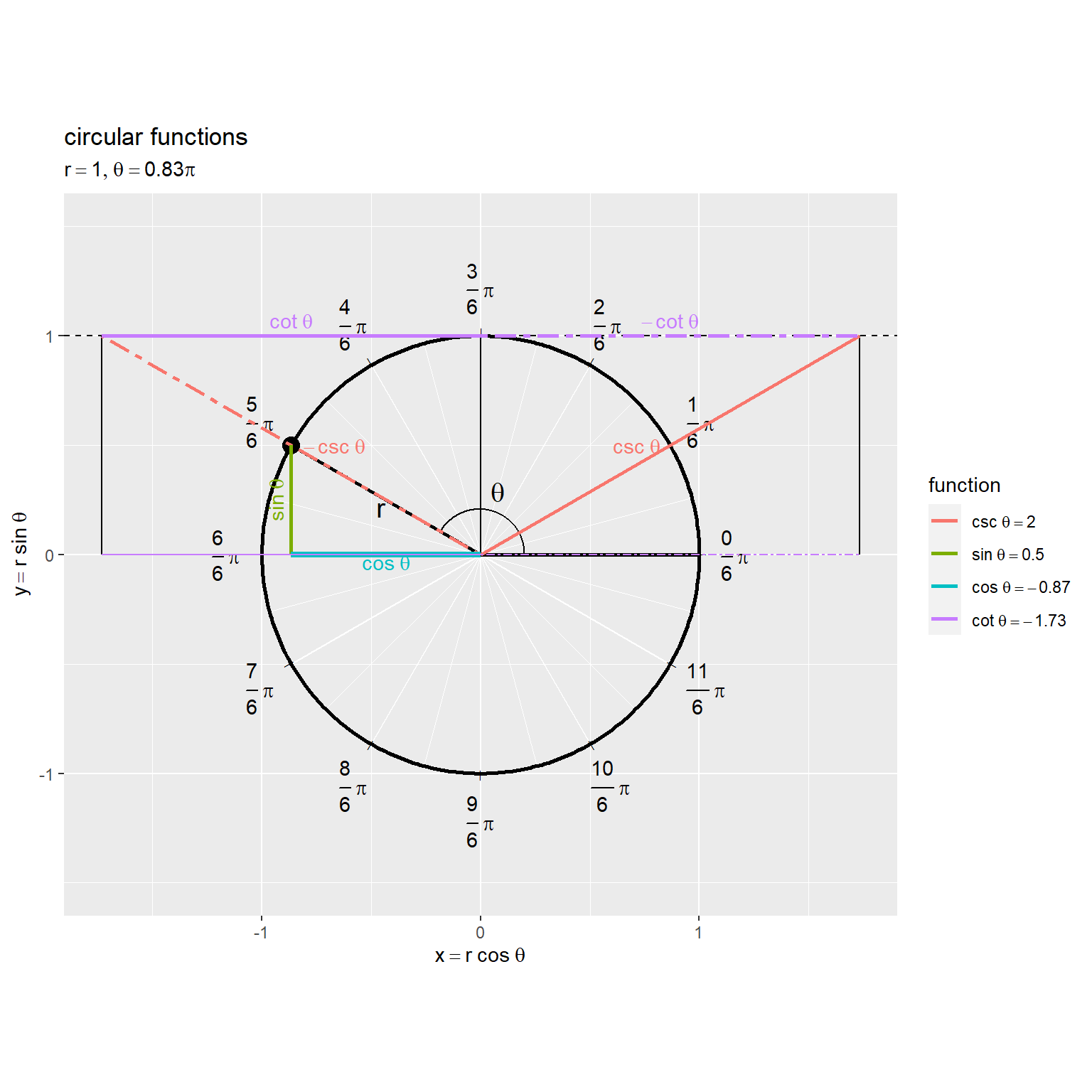
偏角(始線から動径までの反時計回りの角度)を として、単位円(
の円)の円周上の点の座標は
です。
csc関数の定義式 や、この図の相似な直角三角形から、
なのが分かります。
に関する直角三角形について、対辺(
に対応する辺)が1になるように拡大したときの斜辺(
に対応する辺)と言えます。
csc関数の値は、「原点と点 を通る半直線」と「
の直線」の交点
と原点を結ぶ線分の符号付きの長さです。(この図では、)符号はx座標の符号と対応します。
(x座標の)符号を反転した線分を破線で示します。
パターン2
2つ目の方法では、y軸線上を伸びる線分としてcsc関数を可視化します。
・作図コード(クリックで展開)
偏角を示す線分の描画用のデータフレームを作成します。
# 半径線の終点の座標を作成
radius_df <- tibble::tibble(
  x = c(1, cos(theta)),
  y = c(0, sin(theta))
)
radius_df
# A tibble: 2 × 2
       x     y
   <dbl> <dbl>
1  1       0
2 -0.866   0.5
原点と点 を結ぶ線分(始線)、原点と点
を結ぶ線分(動径)用に、円周上の2点の座標を格納します。原点
の座標は、作図時に引数に直接指定します。
関数を示す線分の描画用のデータフレームを作成します。
# 関数の描画順を指定
fnc_level_vec <- c("csc", "sin", "cos", "cot")

# 関数線分の座標を作成
fnc_seg_df <- tibble::tibble(
  fnc = c(
    "csc",
    "sin", "sin",
    "cos", "cos",
    "cot"
  ) |>
    factor(levels = fnc_level_vec), # 関数カテゴリ
  x_from = c(
    0,
    0, 0,
    0, 0,
    cos(theta)
  ),
  y_from = c(
    0,
    0, 0,
    sin(theta), ifelse(sin(theta) >= 0, yes = 1, no = -1),
    sin(theta)
  ),
  x_to = c(
    0,
    0, abs(sin(theta))*cos(theta),
    cos(theta), abs(sin(theta))*cos(theta),
    0
  ),
  y_to = c(
    1/sin(theta),
    sin(theta), abs(sin(theta))*sin(theta),
    sin(theta), abs(sin(theta))*sin(theta),
    1/sin(theta)
  ),
  w = c(
    "bold",
    "thin", "normal",
    "normal", "normal",
    "normal"
  ) # 重なり対策用
)
fnc_seg_df
# A tibble: 6 × 6
  fnc   x_from y_from   x_to  y_to w
  <fct>  <dbl>  <dbl>  <dbl> <dbl> <chr>
1 csc    0        0    0      2    bold
2 sin    0        0    0      0.5  thin
3 sin    0        0   -0.433  0.25 normal
4 cos    0        0.5 -0.866  0.5  normal
5 cos    0        1   -0.433  0.25 normal
6 cot   -0.866    0.5  0      2    normal
「パターン1」と同様に、線分の座標を格納します。
関数ラベルの描画用のデータフレームを作成します。
# 関数ラベルの座標を作成
fnc_label_df <- tibble::tibble(
  fnc = c("csc", "sin", "cos", "cot") |>
    factor(levels = fnc_level_vec), # 関数カテゴリ
  x = c(
    0,
    0,
    0.5 * cos(theta),
    0.5 * cos(theta)
  ),
  y = c(
    0.5 * 1/sin(theta),
    0.5 * sin(theta),
    sin(theta),
    0.5 * (1/sin(theta) + sin(theta))
  ),
  fnc_label = c("csc~theta", "sin~theta", "cos~theta", "cot~theta"),
  a = c(90,  90,  0,    0),
  h = c(0.5, 0.5, 0.5, -0.2),
  v = c(1,  -0.5, 1,    0.5)
)
fnc_label_df
# A tibble: 4 × 7
  fnc        x     y fnc_label     a     h     v
  <fct>  <dbl> <dbl> <chr>     <dbl> <dbl> <dbl>
1 csc    0      1    csc~theta    90   0.5   1
2 sin    0      0.25 sin~theta    90   0.5  -0.5
3 cos   -0.433  0.5  cos~theta     0   0.5   1
4 cot   -0.433  1.25 cot~theta     0  -0.2   0.5
線分の中点の座標とラベル用の文字列などを格納します。
単位円におけるcsc関数のグラフを作成します。
# グラフサイズの下限値・上限値を指定
axis_lower <- 1.5
axis_upper <- 3

# グラフサイズを設定
axis_x_size <- 1.5
axis_y_min  <- min(-axis_lower, 1/sin(theta)) |> max(-axis_upper)
axis_y_max  <- max(axis_lower, 1/sin(theta)) |> min(axis_upper)

# 単位円における関数線分を作図
ggplot() +
  geom_segment(data = rad_tick_df,
               mapping = aes(x = 0, y = 0, xend = x, yend = y, linewidth = grid),
               color = "white", show.legend = FALSE) + # 角度目盛線
  geom_text(data = rad_tick_df,
            mapping = aes(x = x, y = y, angle = a, label = tick_mark),
            size = 2) + # 角度目盛指示線
  geom_text(data = rad_tick_df,
            mapping = aes(x = label_x, y = label_y, label = rad_label, hjust = h, vjust = v),
            parse = TRUE) + # 角度目盛ラベル
  geom_path(data = circle_df,
            mapping = aes(x = x, y = y),
            linewidth = 1) + # 円周
  geom_segment(data = radius_df,
               mapping = aes(x = 0, y = 0, xend = x, yend = y),
               linewidth = 1) + # 半径線
  geom_path(data = angle_mark_df,
            mapping = aes(x = x, y = y)) + # 角マーク
  geom_text(data = angle_label_df,
            mapping = aes(x = x, y = y),
            label = "theta", parse = TRUE,
            size = 5) + # 角ラベル
  geom_text(mapping = aes(x = 0.5*cos(theta+0.1), y = 0.5*sin(theta+0.1)),
            label = "r", parse = TRUE,
            size = 5) + # 半径ラベル:(θ + αで表示位置を調整)
  geom_point(data = point_df,
             mapping = aes(x = x, y = y),
             size = 4) + # 円周上の点
  geom_vline(xintercept = 0, linetype = "dashed") + # 補助線
  geom_segment(data = fnc_seg_df,
               mapping = aes(x = x_from, y = y_from, xend = x_to, yend = y_to,
                             color = fnc, linewidth = w)) + # 関数線分
  geom_text(data = fnc_label_df,
            mapping = aes(x = x, y = y, label = fnc_label, color = fnc,
                          hjust = h, vjust = v, angle = a),
            parse = TRUE, show.legend = FALSE) + # 関数ラベル
  scale_color_hue(labels = parse(text = fnc_label_vec), name = "function") + # 凡例表示用
  scale_linewidth_manual(breaks = c("bold", "normal", "thin", "major", "minor"),
                         values = c(1.5, 1, 0.5, 0.5, 0.25)) + # 線の重なり対策用, 主・補助目盛線用
  guides(color = guide_legend(override.aes = list(linewidth = 1)),
         linewidth = "none") +
  theme(legend.text.align = 0) +
  coord_fixed(ratio = 1,
              xlim = c(-axis_x_size, axis_x_size),
              ylim = c(axis_y_min, axis_y_max)) +
  labs(title = "circular functions",
       subtitle = parse(text = var_label),
       x = expression(x == r ~ cos~theta),
       y = expression(y == r ~ sin~theta))
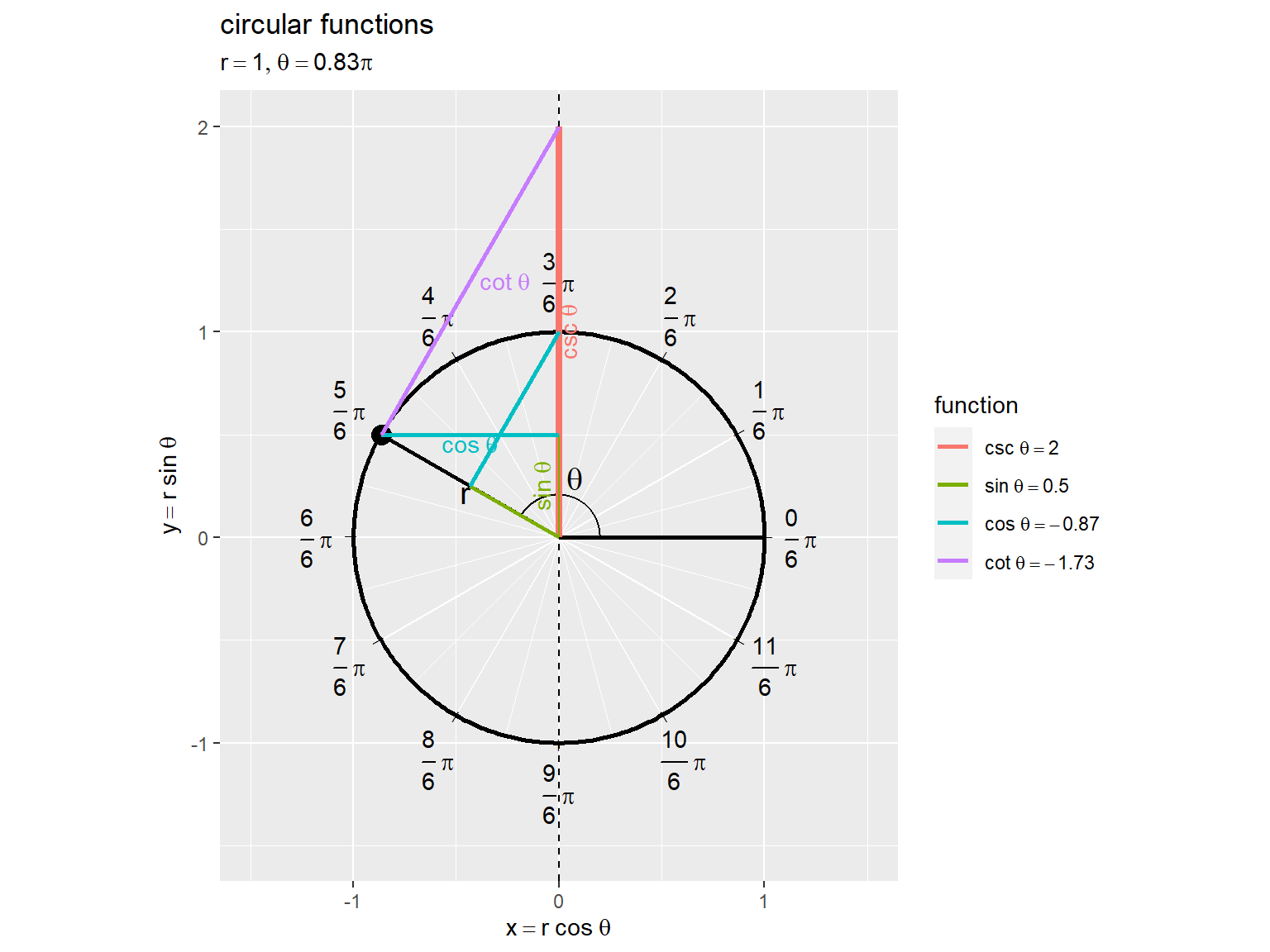
動径(原点と円周上の点を結ぶ線分)を対辺、y軸線の一部を斜辺としたときのパターン1の図と言えます。文字通り首を捻って見てください。
原点を 、円周上の点を
として、「動径に対する点
を通る垂線」と「
の直線」の交点を
とします。csc関数の値は、点
を結ぶ線分の符号付きの長さ(点
のy座標)です。
アニメーションの作成
変数を変化させて、単位円におけるcsc関数のアニメーションを作成します。
作図コードについては「csc_definition.R」を参照してください。
・パターン1
(
は整数)(この図だと
の目盛位置)のとき
なので、動径が水平になり直線
と平行(交点ができない)なため、
を描画(定義)できないのを確認できます。
・パターン2
こちらの図だと、動径の垂線が垂直になり直線 と平行なため、
を描画(定義)できないのが分かります。
単位円と曲線の関係
最後は、単位円と関数曲線のグラフを作成して、変数(ラジアン)と座標の関係を可視化します。
作図コードについては「csc_definition.R」を参照してください。
変数と座標の関係
変数に応じて移動する円周上の点と曲線上の点のアニメーションを作成します。
点の座標
円周上の点とcsc関数曲線上の点の関係を可視化します。
単位円におけるcsc関数の値に関して、x座標の正負に応じて線分を回転し、y軸の値(y軸線上の線分)に変換しています。
のとき曲線が不連続になり、その前後で符号(線分の向き)が変わるのを確認できます。
円周上の点とsin関数・csc関数曲線上の点の関係を可視化します。
左上図でx軸の値(x軸線上の線分)に変換し、さらに左下図によってx座標(横方向の線分)からy座標(縦方向の線分)に変換(回転)し、sin関数とcsc関数の曲線を並べて比較します。
sin関数の値は円周上の点のy座標(符号付きの高さ)です。
円周上の点とsec関数・csc関数曲線上の点の関係を可視化します。
点の推移
円周上を周回した際のcsc関数の推移を可視化します。
単位円を1周する の間隔で、曲線の形状が一致するのを確認できます。
円周上を周回した際のsin関数・csc関数の推移を可視化します。
円周上を周回した際のsec関数・csc関数の推移を可視化します。
この記事では、csc関数の定義を確認しました。次の記事からは、各種パラメータによる波形への影響を確認していきます。または、各種円関数を比較します。
参考書籍
- 『三角関数(改定第3版)』(Newton別冊)ニュートンプレス,2022年.
おわりに
一番わけ分かめな図になってしまった気がしますが、これでも頭を捻って考えたんです。私自身としては一応納得できたのでアップしました。理解の助けになれば幸いです。
作業順としてはこの記事が6つ目です。あとは全部載せを作れば完了です。
2023年7月2日は、Juice=Juiceの元リーダーの金澤朋子さんの28歳のお誕生日です。
かなともならどこでもやっていけるだろうことは想像に難くないけど、楽しく歌っていられる環境だといいな。
- 2024.03.23:加筆修正しました。
面倒臭いー、もう飽きたー、書きたいのはこれからなのにー。
某LLMの影響だと思うのですがここ1年でアクセス数が半減しまして、モチベーションも下がっています。皆さんはもうググらなくなったんですね、私はまだチャピったことがないです。この記事の図とかも言えば作ってくれるんですかね。
私は自分で書かないと理解できない人なのでこれからも書くのですが、面倒なものは面倒です。書きたいこともまだまだあるので、ブログの管理を誰かに任せたい気もします。フロントエンド的な知識も勉強としてやってみたかったのですが、現状では手を出せそうにないので。
ブログという媒体が不要になったとは思ってないのですが、必要な人にまでリーチしてないと思うので、良いなと感じた記事はぜひ宣伝してください!でもアレな界隈まで届いて炎上するのは嫌だー。
【次の内容】