はじめに

　円関数(三角関数)の定義や性質、公式などを可視化して理解しようシリーズです。

　この記事では、arcsec関数のグラフを作成します。

【前の内容】

www.anarchive-beta.com

【他の内容】

www.anarchive-beta.com

【この記事の内容】

はじめに
arcsec関数の定義の可視化
おわりに

arcsec関数の定義の可視化

　arcsec関数(逆sec関数・逆正割関数・逆セカント関数・inverse secant function)の定義をグラフで確認します。sec関数は、円関数(inverse circular functions)・三角関数(inverse trigonometric functions)の1つです。
　sec関数の定義や作図については「【R】sec関数の可視化 - からっぽのしょこ」を参照してください。

　利用するパッケージを読み込みます。

# 利用パッケージ
library(tidyverse)

　この記事では、基本的に パッケージ名::関数名() の記法を使うので、パッケージの読み込みは不要です。ただし、作図コードについてはパッケージ名を省略するので、ggplot2 を読み込む必要があります。
　また、ネイティブパイプ演算子 |> を使います。magrittr パッケージのパイプ演算子 %>% に置き換えられますが、その場合は magrittr を読み込む必要があります。

定義式の確認

　まずは、arcsec関数の定義式を確認します。
　cos関数については「【R】cos関数の可視化 - からっぽのしょこ」、arccos関数については「【R】arccos関数の定義の可視化 - からっぽのしょこ」を参照してください。

arcsec関数とsec関数の関係

　sec関数は、cos関数の逆数で定義されます。

$\displaystyle \sec x = \frac{1}{\cos x}$

　arcsec関数は、sec関数の逆関数で定義されます。

$\displaystyle \mathrm{arcsec}\ x = \sec^{-1} x \quad (x \leq -1\ \mathrm{or}\ 1 \leq x)$

　ただし、定義域は $x \leq -1\ \mathrm{or}\ 1 \leq x$ であり、終域は $0 \leq \mathrm{arcsec}\ x \lt \frac{\pi}{2}\ \mathrm{or}\ \frac{\pi}{2} \lt \mathrm{arcsec}\ x \leq \pi$ です。関数の出力はラジアン(弧度法の角度)、 $\pi$ は円周率です。

arcsec関数とarccos関数の関係

　arcsec関数とarccos関数の関係を導出します。

・途中式(クリックで展開)

　sec関数とcos関数は、逆数の関係でした。

$\displaystyle \sec y = \frac{1}{\cos y} \Leftrightarrow \frac{1}{\sec y} = \cos y$

　cos関数とarccos関数、sec関数とarcsec関数は、それぞれ逆関数の関係でした。

$\displaystyle \begin{aligned} x &= \cos(\arccos x) && (-1 \leq x \leq 1) \\ x &= \sec(\mathrm{arcsec}\ x) && (x \leq -1\ \mathrm{or}\ 1 \leq x) \end{aligned}$

　また、それぞれの関数の定義域と終域より、次の式も成り立ちます。

$\displaystyle \begin{aligned} y &= \arccos(\cos y) && (0 \leq y \lt \pi) \\ y &= \mathrm{arcsec}(\sec y) && (0 \leq y \lt \frac{\pi}{2}\ \mathrm{or}\ \frac{\pi}{2} \lt y \leq \pi) \end{aligned}$

　下の式に関して、 $y = \frac{\pi}{2}$ のとき、 $\cos \frac{\pi}{2} = 0$ になり(0除算になるため) $\sec \frac{\pi}{2}$ を定義できないので、範囲に含まれません。

　これらの式を用いて、arcsec関数とarccos関数の関係を考えます。

逆数によるarccos関数

・途中式(クリックで展開)

　 $x$ を $-1$ 以下または $1$ 以上の値として、arcsec関数を $y$ とおきます。 $y$ は $\frac{\pi}{2}$ を除く $0$ から $\pi$ の値をとります。

$\displaystyle y = \mathrm{arcsec}\ x \tag{1}$

　両辺をsec関数で計算します。

$\displaystyle \begin{aligned} \sec y &= \sec(\mathrm{arcsec}\ x) \\ &= x \end{aligned}$

　逆数の関係より、両辺の逆数をとって、左辺を置き換えます。

$\displaystyle \begin{alignat}{2} && \sec y &= x \\ \Leftrightarrow && \frac{1}{\sec y} &= \frac{1}{x} \\ \Leftrightarrow && \cos y &= \frac{1}{x} \end{alignat}$

　両辺をarccos関数で計算します。

$\displaystyle \arccos(\cos y) = \arccos \frac{1}{x}$

　左辺は

$\displaystyle \arccos(\cos y) = y$

となるので、式(1)で置き換えます。

$\displaystyle \mathrm{arcsec}\ x = \arccos \frac{1}{x} \tag{2}$

　arcsec関数とarccos関数の関係式が得られました。

　また、式(2)より、次の関係も成り立ちます。

$\displaystyle \begin{aligned} \mathrm{arcsec}(\sec z) &= \arccos \left( \frac{1}{\sec z} \right) \\ &= \arccos(\cos z) \end{aligned}$

　以上で、arccos関数を用いてarcsec関数の計算を行えるのが分かりました。

逆数によるarcsec関数

・途中式(クリックで展開)

　同様に、 $x$ を $-1$ から $1$ の値として、arccos関数を $y$ とおきます。 $y$ は $0$ から $\pi$ の値をとります。

$\displaystyle y = \arccos x \tag{3}$

　両辺をcos関数で計算します。

$\displaystyle \begin{aligned} \cos y &= \cos(\arccos x) \\ &= x \end{aligned}$

　逆数の関係より、両辺の逆数をとって、左辺を置き換えます。

$\displaystyle \begin{alignat}{2} && \cos y &= x \\ \Leftrightarrow && \frac{1}{\cos y} &= \frac{1}{x} \\ \Leftrightarrow && \sec y &= \frac{1}{x} \end{alignat}$

　両辺をarcsec関数で計算します。

$\displaystyle \mathrm{arcsec}(\sec y) = \mathrm{arcsec}\ \frac{1}{x}$

　左辺は

$\displaystyle \mathrm{arcsec}(\sec y) = y$

となるので、式(3)で置き換えます。ただし、 $x = 0$ のとき0除算になるため定義できません。また、 $x = 0$ のとき $y = \arccos 0 = \frac{\pi}{2}$ なのでsec関数も定義できません。

$\displaystyle \arccos x = \mathrm{arcsec}\ \frac{1}{x} \tag{4}$

　arccos関数とarcsec関数の関係式が得られました。

　また、式(4)より、次の関係も成り立ちます。

$\displaystyle \begin{aligned} \arccos(\cos z) &= \mathrm{arcsec} \left( \frac{1}{\cos z} \right) \\ &= \mathrm{arcsec}(\sec z) \end{aligned}$

　先ほどの式と一致しました。

　(この記事ではこちらの関係は使いませんが、)arcsec関数を用いてarccos関数の計算を行えるのが分かりました。

曲線の形状

　続いて、arcsec関数のグラフを作成します。

曲線の作成

・作図コード(クリックで展開)

　逆円関数の曲線の描画用のデータフレームを作成します。

# 閾値を指定
threshold <- 4

# 逆関数の曲線の座標を作成
curve_inv_df <- tibble::tibble(
  x        = seq(from = -threshold, to = threshold, length.out = 1001), 
  arcsec_x = acos(1/x), 
  arccsc_x = asin(1/x)
)
curve_inv_df

# A tibble: 1,001 × 3
       x arcsec_x arccsc_x
   <dbl>    <dbl>    <dbl>
 1 -4        1.82   -0.253
 2 -3.99     1.82   -0.253
 3 -3.98     1.82   -0.254
 4 -3.98     1.83   -0.254
 5 -3.97     1.83   -0.255
 6 -3.96     1.83   -0.255
 7 -3.95     1.83   -0.256
 8 -3.94     1.83   -0.256
 9 -3.94     1.83   -0.257
10 -3.93     1.83   -0.257
# ℹ 991 more rows

　sec曲線用の閾値 threshold を指定しておき、閾値の範囲の変数 $x$ と関数 $\mathrm{arcsec}\ x$ の値をデータフレームに格納します。比較用に、 $\mathrm{arccsc}\ x$ の値も格納しておきます。arcsec関数は acos()、arccsc関数は asin() を使って計算できます。

　円関数の曲線の描画用のデータフレームを作成します。

# 元の関数の曲線の座標を作成
curve_df <- tibble::tibble(
  t     = seq(from = -pi, to = pi, length.out = 1001), # ラジアン
  sec_t = 1/cos(t), 
  inv_flag = (t >= 0 & t != 0.5*pi & t <= pi) # 逆関数の終域
) |> 
  dplyr::mutate(
    sec_t = dplyr::if_else(
      (sec_t >= -threshold & sec_t <= threshold), true = sec_t, false = NA_real_
    )
  ) # 閾値外を欠損値に置換
curve_df

# A tibble: 1,001 × 3
       t sec_t inv_flag
   <dbl> <dbl> <lgl>   
 1 -3.14 -1    FALSE   
 2 -3.14 -1.00 FALSE   
 3 -3.13 -1.00 FALSE   
 4 -3.12 -1.00 FALSE   
 5 -3.12 -1.00 FALSE   
 6 -3.11 -1.00 FALSE   
 7 -3.10 -1.00 FALSE   
 8 -3.10 -1.00 FALSE   
 9 -3.09 -1.00 FALSE   
10 -3.09 -1.00 FALSE   
# ℹ 991 more rows

　変数 $-\pi \leq \theta \leq \pi$ と関数 $\sec \theta$ の値をデータフレームに格納します。sec関数は cos() を使って計算できます。
　ただし、 $\theta = (\frac{1}{2} + n) \pi$ ( $n$ は整数)のとき発散するので、閾値 threshold を指定しておき、閾値外の値を(数値型の)欠損値 NA に置き換えます。
　また、 $\theta$ の値が $\mathrm{arcsec}\ x$ のとり得る範囲内かのフラグを inv_flag 列とします。

　arcsec関数とsec関数のグラフを作成します。

・作図コード(クリックで展開)

# ラベル用の文字列を作成
def_label <- paste0(
  "list(", 
  "arcsec~x == sec^{-1}*x, ", 
  "paste(x <= -1 ~or~ x <= 1), ", 
  "0 <= arcsin~x < frac(pi, 2) ~or~ frac(pi, 2) < arcsin~x <= pi", 
  ")"
)

# 関数曲線を作図
ggplot() + 
  geom_segment(mapping = aes(x = c(-Inf, 0), y = c(0, -Inf), 
                             xend = c(Inf, 0), yend = c(0, Inf)), 
               arrow = arrow(length = unit(10, units = "pt"), ends = "last")) + # x・y軸線
  geom_line(data = curve_inv_df, 
            mapping = aes(x = x, y = arcsec_x, color = "arcsec"), 
            linewidth = 1) + # 逆関数
  geom_line(data = curve_df,
            mapping = aes(x = t, y = sec_t, linetype = inv_flag, color = "sec"), 
            linewidth = 1, na.rm = TRUE) + # 元の関数
  geom_abline(slope = 1, intercept = 0, 
              linetype = "dotdash") + # 恒等関数
  scale_color_manual(breaks = c("arcsec", "sec"), 
                     values = c("black", "#F8766D"), 
                     labels = c(expression(arcsec~x), expression(sec~x)), 
                     name = "function") + # 凡例表示用
  scale_linetype_manual(breaks = c(TRUE, FALSE), 
                        values = c("solid", "dotted"), guide ="none") + # 終域用
  coord_fixed(ratio = 1) + # アスペクト比
  labs(title = "inverse secant function", 
       subtitle = parse(text = def_label), 
       x = expression(x), 
       y = expression(f(x)))

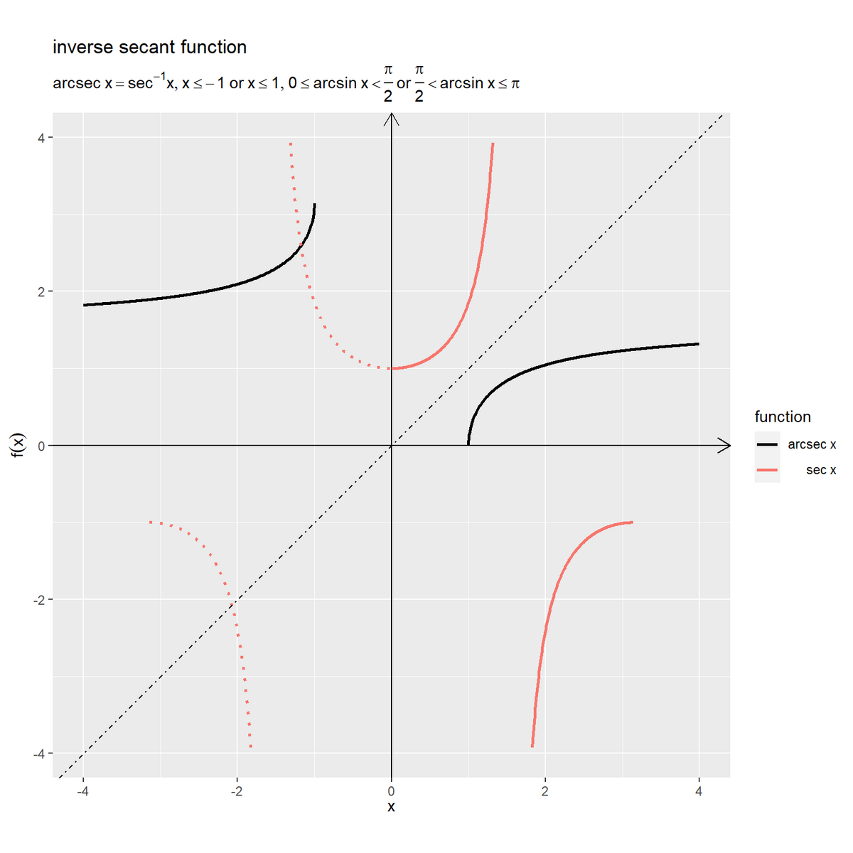
　arcsec関数を実線、sec関数を朱色の実線と点線で、また恒等関数 $f(x) = x$ を鎖線で示します。 $\tau = \mathrm{arcsec}\ x$ がとり得る範囲( $0 \leq \tau \lt \frac{\pi}{2}\ \mathrm{or}\ \frac{\pi}{2} \lt \tau \leq \pi$ )の $\sec \tau$ を実線で示しています。
　恒等関数(傾きが1で切片が0の直線)に対して、arcsec曲線とsec曲線は線対称な曲線です。

　arcsec関数の軸を入れ替えたグラフを作成します。

・作図コード(クリックで展開)

# 範囲πにおける目盛数を指定
tick_num <- 2

# ラジアン軸目盛用の値を作成
rad_break_vec <- seq(from = -pi, to = pi, by = pi/tick_num)
rad_label_vec <- paste(round(rad_break_vec/pi, digits = 2), "* pi")

# 逆関数と元の関数の関係を作図
ggplot() + 
  geom_segment(mapping = aes(x = c(-Inf, 0), y = c(0, -Inf), 
                             xend = c(Inf, 0), yend = c(0, Inf)), 
               arrow = arrow(length = unit(10, units = "pt"), ends = "last")) + # x・y軸線
  geom_vline(xintercept = 0.5*pi, 
             linetype = "twodash") + # 漸近線
  geom_path(data = curve_inv_df, 
            mapping = aes(x = arcsec_x, y = x, color = "arcsec"), 
            linewidth = 1) + # 逆関数
  geom_line(data = curve_df,
            mapping = aes(x = t, y = sec_t, color = "sec"), 
            linewidth = 1, linetype = "dashed") + # 元の関数
  scale_color_manual(breaks = c("arcsec", "sec"), 
                     values = c("black", "#F8766D"), 
                     labels = c(expression(arcsec~x), expression(sec~theta)), 
                     name = "function") + # 凡例表示用
  scale_x_continuous(breaks = rad_break_vec, 
                     labels = parse(text = rad_label_vec)) + # ラジアン軸目盛
  coord_fixed(ratio = 1) + # アスペクト比
  labs(title = "inverse secant function", 
       subtitle = parse(text = def_label), 
       x = expression(list(theta, tau == arcsec~x)), 
       y = expression(x == sec~theta == sec~tau))

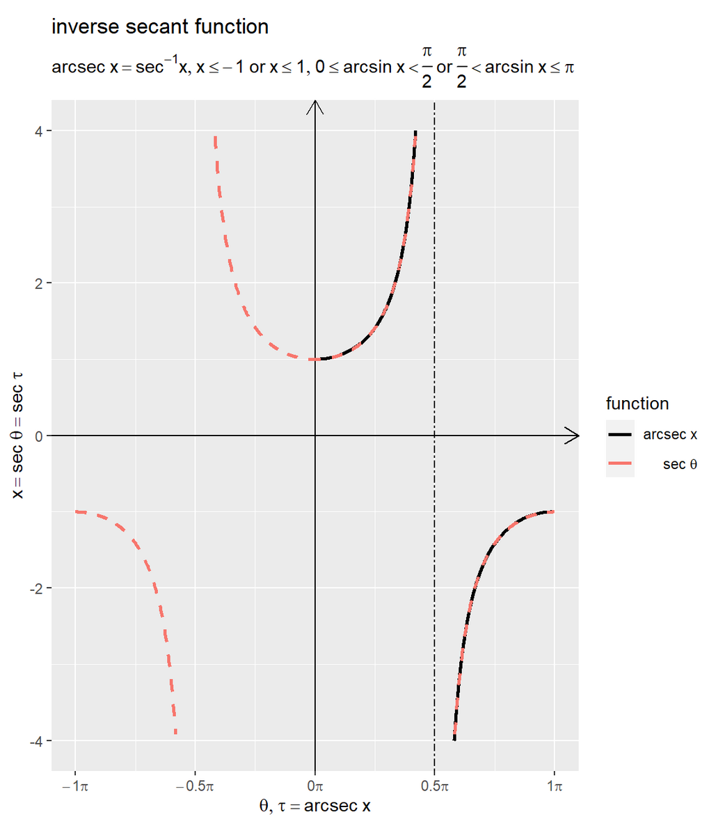
　漸近線を鎖線で示します。
　arcsec曲線の横軸と縦軸を入れ替える(恒等関数の直線に対して反転する)と、sec曲線に一致します。

　arcsec関数とarcsec関数のグラフを作成します。

・作図コード(クリックで展開)

# ラベル用の文字列を作成
def_label <- "arcsec~x == frac(pi, 2) - arccsc~x"

# 関数曲線を作図
ggplot() + 
  geom_segment(mapping = aes(x = c(-Inf, 0), y = c(0, -Inf), 
                             xend = c(Inf, 0), yend = c(0, Inf)), 
               arrow = arrow(length = unit(10, units = "pt"), ends = "last")) + # x・y軸線
  geom_hline(yintercept = 0.5*pi, 
             linetype = "dashed") + # 余角用の水平線
  geom_line(data = curve_inv_df,
            mapping = aes(x = x, y = arcsec_x, linetype = "arcsec"), 
            linewidth = 1) + # arcsec関数
  geom_line(data = curve_inv_df, 
            mapping = aes(x = x, y = arccsc_x, linetype = "arccsc"), 
            linewidth = 1) + # arccsc関数
  scale_linetype_manual(breaks = c("arcsec", "arccsc"), 
                        values = c("solid", "dotted"), 
                        labels = c(expression(arcsec~x), expression(arccsc~x)), 
                        name = "function") + # 凡例表示用
  scale_y_continuous(breaks = rad_break_vec, 
                     labels = parse(text = rad_label_vec)) + # ラジアン軸目盛
  guides(linetype = guide_legend(override.aes = list(linewidth = 0.5))) + # 凡例の体裁
  coord_fixed(ratio = 1, 
              ylim = c(-pi, pi)) + # アスペクト比
  labs(title = "inverse secant function", 
       subtitle = parse(text = def_label), 
       x = expression(x), 
       y = expression(theta == f(x)))

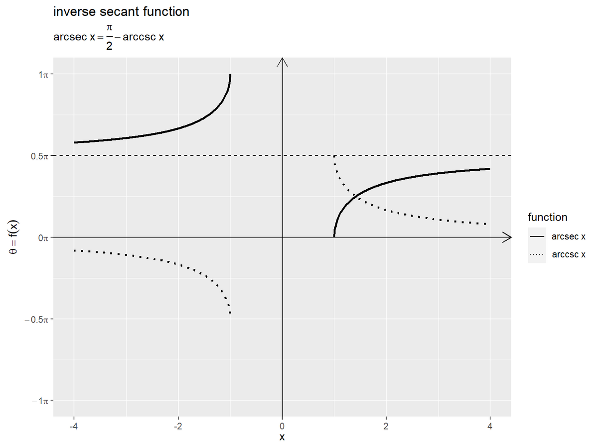
　余角の関係より、 $\mathrm{arcsec}\ x = \frac{\pi}{2} - \mathrm{arccsc}\ x$ が成り立ちます。

単位円と関数の関係

　次は、単位円における偏角(単位円上の点)と円関数(sec・sin・cos・tan)と逆円関数(arcsec)の関係を確認します。
　各関数についてはそれぞれの記事を参照してください。

グラフの作成

　変数を固定して、単位円におけるsec関数の線分とarcsec関数の円弧のグラフを作成します。

・作図コード(クリックで展開)

　円関数の変数を指定して、逆円関数を計算します。

# 点用のラジアンを指定
theta <- 10/6 * pi

# 終域内のラジアンに変換
tau <- acos(cos(theta))
tau / pi

[1] 0.3333333

　sec関数の変数 $\theta$ を指定して、sec関数 $z = \sec \theta$ を変数としてarcsec関数 $\tau = \mathrm{arcsec}\ z$ を計算します。 $\tau = \arccos(\cos \theta)$ で計算できます。

　円周上の点の描画用のデータフレームを作成します。

# 円周上の点の座標を作成
point_df <- tibble::tibble(
  angle = c("theta", "tau"), # 角度カテゴリ
  t = c(theta, tau), 
  x = cos(t), 
  y = sin(t), 
  point_type = c("main", "sub") # 入出力用
)
point_df

# A tibble: 2 × 5
  angle     t     x      y point_type
  <chr> <dbl> <dbl>  <dbl> <chr>     
1 theta  5.24   0.5 -0.866 main      
2 tau    1.05   0.5  0.866 sub

　円関数の入力 $\theta$ と逆円関数の出力 $\tau$ それぞれについて、単位円上の点の座標 $(x, y) = (\cos t, \sin t)$ を計算します。

　単位円の描画用のデータフレームを作成します。

# 単位円の座標を作成
circle_df <- tibble::tibble(
  t = seq(from = 0, to = 2*pi, length.out = 361), # 1周期分のラジアン
  r = 1, # 半径
  x = r * cos(t), 
  y = r * sin(t)
)

# 範囲πにおける目盛数を指定
tick_num <- 6

# 角度目盛の座標を作成
rad_tick_df <- tibble::tibble(
  i = seq(from = 0, to = 2*tick_num-0.5, by = 0.5), # 目盛番号
  t = i/tick_num * pi, # ラジアン
  r = 1, # 半径
  x = r * cos(t), 
  y = r * sin(t), 
  major_flag = i%%1 == 0, # 主・補助フラグ
  grid       = dplyr::if_else(major_flag, true = "major", false = "minor") # 目盛カテゴリ
)

　円周と角度軸目盛の座標を作成します。

　偏角の描画用のデータフレームを作成します。

# 半径線の終点の座標を作成
radius_df <- dplyr::bind_rows(
  # 始線
  tibble::tibble(
    x = 1, 
    y = 0, 
    line_type = "main" # 入出力用
  ), 
  # 動径
  point_df |> 
    dplyr::select(x, y, line_type = point_type)
)

# 角マークの座標を作成
d_in  <- 0.2
d_spi <- 0.005
d_out <- 0.3
angle_mark_df <- dplyr::bind_rows(
  # 元の関数の入力
  tibble::tibble(
    angle = "theta", # 角度カテゴリ
    u = seq(from = 0, to = theta, length.out = 600), 
    x = (d_in + d_spi*u) * cos(u), 
    y = (d_in + d_spi*u) * sin(u)
  ), 
  # 逆関数の出力
  tibble::tibble(
    angle = "tau", # 角度カテゴリ
    u = seq(from = 0, to = tau, length.out = 600), 
    x = d_out * cos(u), 
    y = d_out * sin(u)
  )
)

# 角ラベルの座標を作成
d_in  <- 0.1
d_out <- 0.4
angle_label_df <- tibble::tibble(
  u = 0.5 * c(theta, tau), 
  x = c(d_in, d_out) * cos(u), 
  y = c(d_in, d_out) * sin(u), 
  angle_label = c("theta", "tau")
)

　 $\theta, \tau$ それぞれについて、始線と動径、角マークと角ラベルの座標を作成します。

　逆円関数を示す円弧の描画用のデータフレームを作成します。

# 関数円弧の座標を作成
radian_df <- tibble::tibble(
  u = seq(from = 0, to = tau, length.out = 600), 
  r = 1, # 半径
  x = r * cos(u), 
  y = r * sin(u)
)
radian_df

# A tibble: 600 × 4
         u     r     x       y
     <dbl> <dbl> <dbl>   <dbl>
 1 0           1  1    0      
 2 0.00175     1  1.00 0.00175
 3 0.00350     1  1.00 0.00350
 4 0.00524     1  1.00 0.00524
 5 0.00699     1  1.00 0.00699
 6 0.00874     1  1.00 0.00874
 7 0.0105      1  1.00 0.0105 
 8 0.0122      1  1.00 0.0122 
 9 0.0140      1  1.00 0.0140 
10 0.0157      1  1.00 0.0157 
# ℹ 590 more rows

　ラジアン $0 \leq u \leq \tau$ を作成して、単位円の円周上の(半径が $r = 1$ の)円弧の座標 $(x, y) = (\cos u, \sin u)$ を計算します。

　円関数を示す線分の描画用のデータフレームを作成します。

# 関数の描画順を指定
fnc_level_vec <- c("arcsec", "sec", "sin", "cos", "tan")

# 符号の反転フラグを設定
rev_flag <- sin(theta) < 0

# 関数線分の座標を格納
fnc_seg_df <- tibble::tibble(
  fnc = c(
    "sec", "sec", 
    "sin", 
    "cos", 
    "tan", "tan"
  ) |> 
    factor(levels = fnc_level_vec), # 関数カテゴリ用
  x_from = c(
    0, ifelse(test = rev_flag, yes = 0, no = NA), 
    cos(theta), 
    0, 
    1, ifelse(test = rev_flag, yes = 1, no = NA)
  ), 
  y_from = c(
    0, ifelse(test = rev_flag, yes = 0, no = NA), 
    0, 
    0, 
    0, ifelse(test = rev_flag, yes = 0, no = NA)
  ), 
  x_to = c(
    1, ifelse(test = rev_flag, yes = 1, no = NA), 
    cos(theta), 
    cos(theta), 
    1, ifelse(test = rev_flag, yes = 1, no = NA)
  ), 
  y_to = c(
    ifelse(test = rev_flag, yes = -tan(theta), no = tan(theta)), ifelse(test = rev_flag, yes = tan(theta), no = NA), 
    sin(theta), 
    0, 
    tan(theta), ifelse(test = rev_flag, yes = -tan(theta), no = NA)
  ), 
  line_type = c(
    "main", "sub", 
    "main", 
    "main", 
    "main", "sub"
  ) # 符号の反転用
)
fnc_seg_df

# A tibble: 6 × 6
  fnc   x_from y_from  x_to   y_to line_type
  <fct>  <dbl>  <dbl> <dbl>  <dbl> <chr>    
1 sec      0        0   1    1.73  main     
2 sec      0        0   1   -1.73  sub      
3 sin      0.5      0   0.5 -0.866 main     
4 cos      0        0   0.5  0     main     
5 tan      1        0   1   -1.73  main     
6 tan      1        0   1    1.73  sub

　各線分に対応する関数カテゴリを fnc 列として線の描き分けなどに使います。線分の描画順(重なり順や色付け順)を因子レベルで設定します。
　各線分の始点の座標を x_from, y_from 列、終点の座標を x_to, y_to 列として、完成図を見ながら頑張って格納します。

　関数ラベルの描画用のデータフレームを作成します。

# 関数ラベルの座標を格納
fnc_label_df <- tibble::tibble(
  fnc = c(
    "arcsec", 
    "sec", "sec", 
    "sin", 
    "cos", 
    "tan", "tan"
  ) |> 
    factor(levels = fnc_level_vec), # 関数カテゴリ
  x = c(
    cos(0.5 * tau), 
    0.5, ifelse(test = rev_flag, yes = 0.5, no = NA), 
    cos(theta), 
    0.5 * cos(theta), 
    1, ifelse(test = rev_flag, yes = 1, no = NA)
  ), 
  y = c(
    sin(0.5 * tau), 
    0.5 * ifelse(test = rev_flag, yes = -tan(theta), no = tan(theta)), ifelse(test = rev_flag, yes = 0.5*tan(theta), no = NA), 
    0.5 * sin(theta), 
    0, 
    0.5 * tan(theta), ifelse(test = rev_flag, yes = -0.5*tan(theta), no = NA)
  ), 
  fnc_label = c(
    "arcsec(sec~theta)", 
    "sec~theta", "-sec~theta", 
    "sin~theta", 
    "cos~theta", 
    "tan~theta", "-tan~theta"
  ), 
  a = c(
    0, 
    0, 0, 
    90, 
    0, 
    90, 90
  ), 
  h = c(
    -0.1, 
    1.2, 1.2, 
    0.5, 
    0.5, 
    0.5, 0.5
  ), 
  v = c(
    -0.5, 
    0.5, 0.5, 
    -0.5, 
    1, 
    1, 1
  )
)
fnc_label_df

# A tibble: 7 × 7
  fnc        x      y fnc_label             a     h     v
  <fct>  <dbl>  <dbl> <chr>             <dbl> <dbl> <dbl>
1 arcsec 0.866  0.5   arcsec(sec~theta)     0  -0.1  -0.5
2 sec    0.5    0.866 sec~theta             0   1.2   0.5
3 sec    0.5   -0.866 -sec~theta            0   1.2   0.5
4 sin    0.5   -0.433 sin~theta            90   0.5  -0.5
5 cos    0.25   0     cos~theta             0   0.5   1  
6 tan    1     -0.866 tan~theta            90   0.5   1  
7 tan    1      0.866 -tan~theta           90   0.5   1

　関数ごとに1つの線分の中点に関数名を表示することにします。
　ラベルの表示角度を a 列、表示角度に応じた左右の表示位置を h 列、上下の表示位置を v 列として指定します。

　単位円におけるarcsec関数のグラフを作成します。

# ラベル用の文字列を作成
var_label <- paste0(
  "list(", 
  "r == 1, ", 
  "theta == ", round(theta/pi, digits = 2), " * pi, ", 
  "tau == ", round(tau/pi, digits = 2), " * pi", 
  ")"
)
fnc_label_vec <- paste(
  c("arcsec(sec~theta)", "sec~theta", "sin~theta", "cos~theta", "tan~theta"), 
  c(tau, 1/cos(theta), sin(theta), cos(theta), tan(theta)) |> 
    round(digits = 2), 
  sep = " == "
)

# グラフサイズの下限値・上限値を指定
axis_lower <- 1.5
axis_upper <- 3

# グラフサイズを設定
axis_x_size <- 1.5
axis_y_size <- max(axis_lower, abs(tan(theta))) |> min(axis_upper)

# 単位円における関数線分を作図
ggplot() + 
  geom_segment(data = rad_tick_df, 
               mapping = aes(x = 0, y = 0, xend = x, yend = y, linewidth = grid), 
               color = "white", show.legend = FALSE) + # θ軸目盛線
  geom_segment(mapping = aes(x = c(-Inf, 0), y = c(0, -Inf), 
                             xend = c(Inf, 0), yend = c(0, Inf)),
               arrow = arrow(length = unit(10, units = "pt"), ends = "last")) + # x・y軸線
  geom_path(data = circle_df, 
            mapping = aes(x = x, y = y), 
            linewidth = 1) + # 円周
  geom_segment(data = radius_df, 
               mapping = aes(x = 0, y = 0, xend = x, yend = y, 
                             linewidth = line_type, linetype = line_type), 
               show.legend = FALSE) + # 半径線
  geom_path(data = angle_mark_df, 
            mapping = aes(x = x, y = y, group = angle)) + # 角マーク
  geom_text(data = angle_label_df, 
            mapping = aes(x = x, y = y, label = angle_label), 
            parse = TRUE, size = 5) + # 角ラベル
  geom_text(mapping = aes(x = 0.5*cos(theta+0.1), y = 0.5*sin(theta+0.1)), 
            label = "r", parse = TRUE, 
            size = 5) + # 半径ラベル:(θ + αで表示位置を調整)
  geom_point(data = point_df, 
             mapping = aes(x = x, y = y, shape = point_type), 
             size = 4, show.legend = FALSE) + # 円周上の点
  geom_segment(mapping = aes(x = cos(theta), y = sin(theta), 
                             xend = cos(tau), yend = sin(tau)), 
               linetype = "dotted") + # 動径間の補助線
  geom_vline(xintercept = 1, linetype = "dashed") + # 補助線
  geom_path(data = radian_df, 
            mapping = aes(x = x, y = y), 
            color = "red", linewidth = 1) + # 関数円弧
  geom_segment(data = fnc_seg_df, 
               mapping = aes(x = x_from, y = y_from, xend = x_to, yend = y_to, 
                             color = fnc, linetype = line_type), 
               linewidth = 1) + # 関数線分
  geom_text(data = fnc_label_df,
            mapping = aes(x = x, y = y, label = fnc_label, color = fnc,
                          angle = a, hjust = h, vjust = v),
            parse = TRUE, show.legend = FALSE) + # 関数ラベル
  scale_color_manual(breaks = fnc_level_vec, 
                     values = c("red", scales::hue_pal()(n = length(fnc_level_vec)-1)), 
                     labels = parse(text = fnc_label_vec), name = "function") + # 凡例表示用, 色の共通化用
  scale_shape_manual(breaks = c("main", "sub"), 
                     values = c("circle", "circle open")) + # 入出力用
  scale_linetype_manual(breaks = c("main", "sub"), 
                        values = c("solid", "dashed")) + # 補助線用
  scale_linewidth_manual(breaks = c("main", "sub", "major", "minor"), 
                         values = c(1, 0.5, 0.5, 0.25)) + # 補助線用, 主・補助目盛線用
  guides(linewidth = "none", linetype = "none") + 
  theme(legend.text.align = 0) + 
  coord_fixed(ratio = 1, 
              xlim = c(-axis_x_size, axis_x_size), 
              ylim = c(-axis_y_size, axis_y_size)) + 
  labs(title = "circular functions", 
       subtitle = parse(text = var_label), 
       x = expression(x == r ~ cos~theta), 
       y = expression(y == r ~ sin~theta))

　(y座標の)符号を反転した線分を破線で示します。
　偏角(x軸の正の部分からの角度)をラジアン $\theta$ とします。中心角が $\theta$ の弧長は $l = r \theta$ です。よって(ラジアンを用いると)、単位円における( $r = 1$ のとき)偏角 $\theta$ と弧長 $l$ が一致します。半径が $r$ の円周上の点の座標は $(x, y) = (r \cos \theta, r \sin \theta)$ です。
　sec関数の値を $z = \sec \theta$ 、arcsec関数の値を $\tau = \mathrm{arcsec} z$ と置く(sec関数の入力を $\theta$ 、arcsec関数の出力を $\tau$ とする)と、sec関数が $z$ になる偏角(弧長)が $\tau$ であり、 $\sec \theta = \sec \tau$ となります。

アニメーションの作成

　変数を変化させて、単位円におけるarcsec関数のアニメーションを作成します。
　作図コードについては「GitHub - anemptyarchive/Mathematics/.../arcsec_definition.R」を参照してください。

　単位円における偏角とarcsec関数の円弧の関係を可視化します。

　sec関数の終域 $\sec \theta \leq -1\ \mathrm{or}\ 1 \leq \sec \theta$ をarcsec関数の定義域 $z \leq -1\ \mathrm{or}\ 1 \leq z$ として、終域が $0 \leq \mathrm{arcsec}\ z \lt \frac{\pi}{2}\ \mathrm{or}\ \frac{\pi}{2} \lt \mathrm{arcsec}\ z \leq \pi$ ( $\cos \frac{\pi}{2} = 0$ なので(0除算になるので)sec関数とtan関数が定義できない $\frac{\pi}{2}$ を除く $0$ から $\pi$ の範囲) になるのを確認できます。
　 $n$ を整数として $\theta = (\frac{1}{2} + n) \pi$ のとき、sec関数とtan関数を示す線が平行になり(半直線)になるためそれぞれ定義できません。