はじめに

　円関数(三角関数)の定義や性質、公式などを可視化して理解しようシリーズです。

　この記事では、arccsc関数のグラフを作成します。

【前の内容】

www.anarchive-beta.com

【他の内容】

www.anarchive-beta.com

【この記事の内容】

はじめに
arccsc関数の定義の可視化
おわりに

arccsc関数の定義の可視化

　arccsc関数(逆csc関数・逆余割関数・逆コセカント関数・inverse cosecant function)の定義をグラフで確認します。csc関数は、円関数(inverse circular functions)・三角関数(inverse trigonometric functions)の1つです。
　csc関数の定義や作図については「【R】csc関数の可視化 - からっぽのしょこ」を参照してください。

　利用するパッケージを読み込みます。

# 利用パッケージ
library(tidyverse)

　この記事では、基本的に パッケージ名::関数名() の記法を使うので、パッケージの読み込みは不要です。ただし、作図コードについてはパッケージ名を省略するので、ggplot2 を読み込む必要があります。
　また、ネイティブパイプ演算子 |> を使います。magrittr パッケージのパイプ演算子 %>% に置き換えられますが、その場合は magrittr を読み込む必要があります。

定義式の確認

　まずは、arccsc関数の定義式を確認します。
　sin関数については「【R】sin関数の可視化 - からっぽのしょこ」、arcsin関数については「【R】arcsin関数の定義の可視化 - からっぽのしょこ」を参照してください。

arccsc関数とcsc関数の関係

　csc関数は、sin関数の逆数で定義されます。

$\displaystyle \csc x = \frac{1}{\sin x}$

　arccsc関数は、csc関数の逆関数で定義されます。

$\displaystyle \mathrm{arccsc}\ x = \csc^{-1} x \quad (x \leq -1\ \mathrm{or}\ 1 \leq x)$

　ただし、定義域は $x \leq -1\ \mathrm{or}\ 1 \leq x$ であり、終域は $-\frac{\pi}{2} \leq \mathrm{arccsc}\ x \lt 0\ \mathrm{or}\ 0 \lt \mathrm{arccsc}\ x \leq \frac{\pi}{2}$ です。関数の出力はラジアン(弧度法の角度)、 $\pi$ は円周率です。

arccsc関数とarcsin関数の関係

　arcsec関数とarccos関数の関係を導出します。

・途中式(クリックで展開)

　csc関数とsin関数は、逆数の関係でした。

$\displaystyle \csc y = \frac{1}{\sin y} \Leftrightarrow \frac{1}{\csc y} = \sin y$

　sin関数とarcsin関数、csc関数とarccsc関数は、それぞれ逆関数の関係でした。

$\displaystyle \begin{aligned} x &= \sin(\arcsin x) && (-1 \leq x \leq 1) \\ x &= \csc(\mathrm{arccsc}\ x) && (x \leq -1\ \mathrm{or}\ 1 \leq x) \end{aligned}$

　また、それぞれの関数の定義域と終域より、次の式も成り立ちます。

$\displaystyle \begin{aligned} y &= \arcsin(\sin y) && (-\frac{\pi}{2} \leq y \lt \frac{\pi}{2}) \\ y &= \mathrm{arccsc}(\csc y) && (-\frac{\pi}{2} \leq y \lt 0\ \mathrm{or}\ 0 \lt y \leq \frac{\pi}{2}) \end{aligned}$

　下の式に関して、 $y = 0$ のとき、 $\sin 0 = 0$ になり(0除算になるため) $\csc 0$ を定義できないので、範囲に含まれません。

　これらの式を用いて、arccsc関数とarcsin関数の関係を考えます。

逆数によるarcsin関数

・途中式(クリックで展開)

　 $x$ を $-1$ 以下または $1$ 以上の値として、arccsc関数を $y$ とおきます。 $y$ は $0$ を除く $-\frac{\pi}{2}$ から $\frac{\pi}{2}$ の値をとります。

$\displaystyle y = \mathrm{arccsc}\ x \tag{1}$

　両辺をcsc関数で計算します。

$\displaystyle \begin{aligned} \csc y &= \csc(\mathrm{arccsc}\ x) \\ &= x \end{aligned}$

　逆数の関係より、両辺の逆数をとって、左辺を置き換えます。

$\displaystyle \begin{alignat}{2} && \csc y &= x \\ \Leftrightarrow && \frac{1}{\csc y} &= \frac{1}{x} \\ \Leftrightarrow && \sin y &= \frac{1}{x} \end{alignat}$

　両辺をarcsin関数で計算します。

$\displaystyle \arcsin(\sin y) = \arcsin \frac{1}{x}$

　左辺は

$\displaystyle \arcsin(\sin y) = y$

となるので、式(1)で置き換えます。

$\displaystyle \mathrm{arccsc}\ x = \arcsin \frac{1}{x} \tag{2}$

　arccsc関数とarcsin関数の関係式が得られました。

　また、式(2)より、次の関係も成り立ちます。

$\displaystyle \begin{aligned} \mathrm{arccsc}(\csc z) &= \arcsin \left( \frac{1}{\csc z} \right) \\ &= \arcsin(\sin z) \end{aligned}$

　以上で、arcsin関数を用いてarccsc関数の計算を行えるのが分かりました。

逆数によるarccsc関数

・途中式(クリックで展開)

　同様に、 $x$ を $-1$ から $1$ の値として、arcsin関数を $y$ とおきます。 $y$ は $-\frac{\pi}{2}$ から $\frac{\pi}{2}$ の値をとります。

$\displaystyle y = \arcsin x \tag{3}$

　両辺をsin関数で計算します。

$\displaystyle \begin{aligned} \sin y &= \sin(\arcsin x) \\ &= x \end{aligned}$

　逆数の関係より、両辺の逆数をとって、左辺を置き換えます。

$\displaystyle \begin{alignat}{2} && \sin y &= x \\ \Leftrightarrow && \frac{1}{\sin y} &= \frac{1}{x} \\ \Leftrightarrow && \csc y &= \frac{1}{x} \end{alignat}$

　両辺をarccsc関数で計算します。

$\displaystyle \mathrm{arccsc}(\csc y) = \mathrm{arccsc}\ \frac{1}{x}$

　左辺は

$\displaystyle \mathrm{arccsc}(\csc y) = y$

となるので、式(3)で置き換えます。ただし、 $x = 0$ のとき0除算になるため定義できません。また、 $x = 0$ のとき $y = \arcsin 0 = 0$ なのでcsc関数も定義できません。

$\displaystyle \arcsin x = \mathrm{arccsc}\ \frac{1}{x} \tag{4}$

　arcsin関数とarccsc関数の関係式が得られました。

　また、式(4)より、次の関係も成り立ちます。

$\displaystyle \begin{aligned} \arcsin(\sin z) &= \mathrm{arccsc} \left( \frac{1}{\sin z} \right) \\ &= \mathrm{arccsc}(\csc z) \end{aligned}$

　先ほどの式と一致しました。

　(この記事ではこちらの関係は使いませんが、)arccsc関数を用いてarcsin関数の計算を行えるのが分かりました。

曲線の形状

　続いて、arccsc関数のグラフを作成します。

曲線の作成

・作図コード(クリックで展開)

　逆円関数の曲線の描画用のデータフレームを作成します。

# 閾値を指定
threshold <- 4

# 逆関数の曲線の座標を作成
curve_inv_df <- tibble::tibble(
  x        = seq(from = -threshold, to = threshold, length.out = 1001), 
  arccsc_x = asin(1/x), 
  arcsec_x = acos(1/x)
)
curve_inv_df

# A tibble: 1,001 × 3
       x arccsc_x arcsec_x
   <dbl>    <dbl>    <dbl>
 1 -4      -0.253     1.82
 2 -3.99   -0.253     1.82
 3 -3.98   -0.254     1.82
 4 -3.98   -0.254     1.83
 5 -3.97   -0.255     1.83
 6 -3.96   -0.255     1.83
 7 -3.95   -0.256     1.83
 8 -3.94   -0.256     1.83
 9 -3.94   -0.257     1.83
10 -3.93   -0.257     1.83
# ℹ 991 more rows

　csc曲線用の閾値 threshold を指定しておき、閾値の範囲の変数 $x$ と関数 $\mathrm{arccsc}\ x$ の値をデータフレームに格納します。比較用に、 $\mathrm{arcsec}\ x$ の値も格納しておきます。arccsc関数は asin()、arcsec関数は acos() を使って計算できます。

　円関数の曲線の描画用のデータフレームを作成します。

# 元の関数の曲線の座標を作成
curve_df <- tibble::tibble(
  t     = seq(from = -pi, to = pi, length.out = 1001), # ラジアン
  csc_t = 1/sin(t), 
  inv_flag = (t >= -0.5*pi & t != 0 & t <= 0.5*pi) # 逆関数の終域
) |> 
  dplyr::mutate(
    csc_t = dplyr::if_else(
      (csc_t >= -threshold & csc_t <= threshold), true = csc_t, false = NA_real_
    )
  ) # 閾値外を欠損値に置換
curve_df

# A tibble: 1,001 × 3
       t csc_t inv_flag
   <dbl> <dbl> <lgl>   
 1 -3.14    NA FALSE   
 2 -3.14    NA FALSE   
 3 -3.13    NA FALSE   
 4 -3.12    NA FALSE   
 5 -3.12    NA FALSE   
 6 -3.11    NA FALSE   
 7 -3.10    NA FALSE   
 8 -3.10    NA FALSE   
 9 -3.09    NA FALSE   
10 -3.09    NA FALSE   
# ℹ 991 more rows

　変数 $-\pi \leq \theta \leq \pi$ と関数 $\csc \theta$ の値をデータフレームに格納します。csc関数は sin() を使って計算できます。
　ただし、 $\theta = n \pi$ ( $n$ は整数)のとき発散するので、閾値 threshold を指定しておき、閾値外の値を(数値型の)欠損値 NA に置き換えます。
　また、 $\theta$ の値が $\mathrm{arccsc}\ x$ のとり得る範囲内かのフラグを inv_flag 列とします。

　arccsc関数とcsc関数のグラフを作成します。

・作図コード(クリックで展開)

# ラベル用の文字列を作成
def_label <- paste0(
  "list(", 
  "arcscsc~x == csc^{-1}*x, ", 
  "paste(x <= -1 ~or~ x <= 1), ", 
  "-frac(pi, 2) <= arccsc~x < 0 ~or~ 0 < arccsc~x <= frac(pi, 2)", 
  ")"
)

# 関数曲線を作図
ggplot() + 
  geom_segment(mapping = aes(x = c(-Inf, 0), y = c(0, -Inf), 
                             xend = c(Inf, 0), yend = c(0, Inf)), 
               arrow = arrow(length = unit(10, units = "pt"), ends = "last")) + # x・y軸線
  geom_line(data = curve_inv_df, 
            mapping = aes(x = x, y = arccsc_x, color = "arccsc"), 
            linewidth = 1) + # 逆関数
  geom_line(data = curve_df,
            mapping = aes(x = t, y = csc_t, linetype = inv_flag, color = "csc"), 
            linewidth = 1, na.rm = TRUE) + # 元の関数
  geom_abline(slope = 1, intercept = 0, 
              linetype = "dotdash") + # 恒等関数
  scale_color_manual(breaks = c("arccsc", "csc"), 
                     values = c("black", "#F8766D"), 
                     labels = c(expression(arccsc~x), expression(csc~x)), 
                     name = "function") + # 凡例表示用
  scale_linetype_manual(breaks = c(TRUE, FALSE), 
                        values = c("solid", "dotted"), guide ="none") + # 終域用
  coord_fixed(ratio = 1) + # アスペクト比
  labs(title = "inverse cosecant function", 
       subtitle = parse(text = def_label), 
       x = expression(x), 
       y = expression(f(x)))

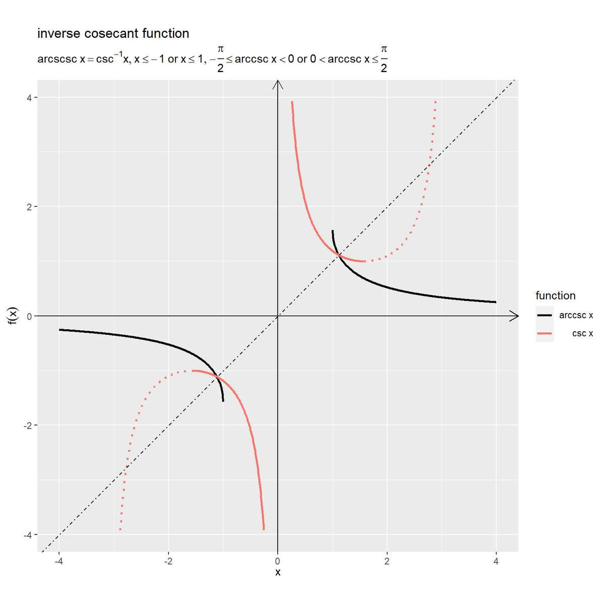
　arccsc関数を実線、csc関数を朱色の実線と点線で、また恒等関数 $f(x) = x$ を鎖線で示します。 $\tau = \mathrm{arccsc}\ x$ がとり得る範囲( $-\frac{\pi}{2} \leq \tau \lt 0\ \mathrm{or}\ 0 \lt \tau \leq \frac{\pi}{2}$ )の $\csc \tau$ を実線で示しています。
　恒等関数(傾きが1で切片が0の直線)に対して、arccsc曲線とcsc曲線は線対称な曲線です。

　arccsc関数の軸を入れ替えたグラフを作成します。

・作図コード(クリックで展開)

# 範囲πにおける目盛数を指定
tick_num <- 2

# ラジアン軸目盛用の値を作成
rad_break_vec <- seq(from = -pi, to = pi, by = pi/tick_num)
rad_label_vec <- paste(round(rad_break_vec/pi, digits = 2), "* pi")

# 逆関数と元の関数の関係を作図
ggplot() + 
  geom_segment(mapping = aes(x = c(-Inf, 0), y = c(0, -Inf), 
                             xend = c(Inf, 0), yend = c(0, Inf)), 
               arrow = arrow(length = unit(10, units = "pt"), ends = "last")) + # x・y軸線
  geom_vline(xintercept = 0, 
             linetype = "twodash") + # 漸近線
  geom_path(data = curve_inv_df, 
            mapping = aes(x = arccsc_x, y = x, color = "arccsc"), 
            linewidth = 1) + # 逆関数
  geom_line(data = curve_df,
            mapping = aes(x = t, y = csc_t, color = "csc"), 
            linewidth = 1, linetype = "dashed") + # 元の関数
  scale_color_manual(breaks = c("arccsc", "csc"), 
                     values = c("black", "#F8766D"), 
                     labels = c(expression(arccsc~x), expression(csc~theta)), 
                     name = "function") + # 凡例表示用
  scale_x_continuous(breaks = rad_break_vec, 
                     labels = parse(text = rad_label_vec)) + # ラジアン軸目盛
  coord_fixed(ratio = 1) + # アスペクト比
  labs(title = "inverse cosecant function", 
       subtitle = parse(text = def_label), 
       x = expression(list(theta, tau == arccsc~x)), 
       y = expression(x == csc~theta == csc~tau))

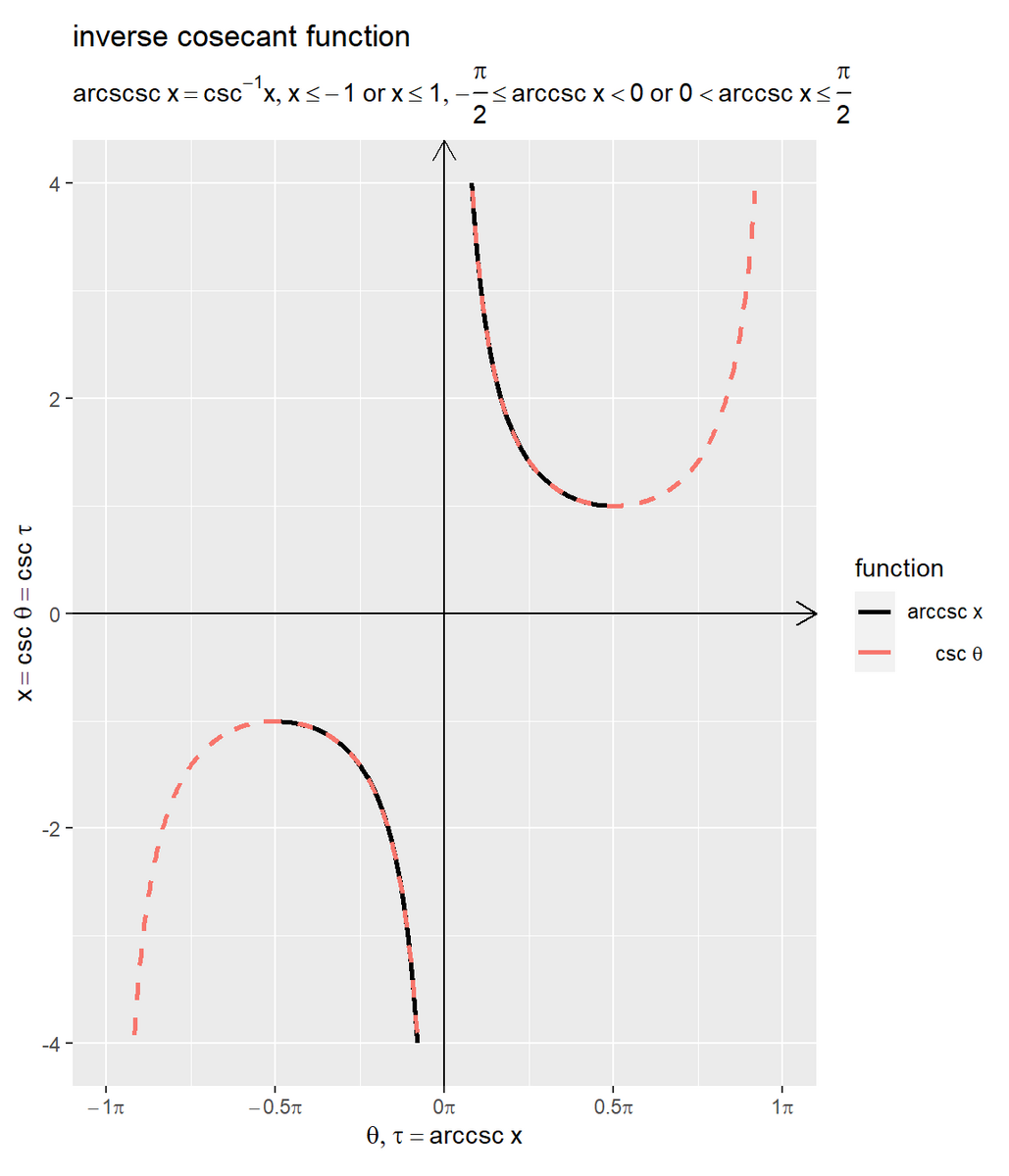
　(縦軸線と重なって見えませんが)漸近線を鎖線で示します。
　arccsc曲線の横軸と縦軸を入れ替える(恒等関数の直線に対して反転する)と、csc曲線に一致します。

　arccsc関数とarcsec関数のグラフを作成します。

・作図コード(クリックで展開)

# ラベル用の文字列を作成
def_label <- "arccsc~x == frac(pi, 2) - arcsec~x"

# 関数曲線を作図
ggplot() + 
  geom_segment(mapping = aes(x = c(-Inf, 0), y = c(0, -Inf), 
                             xend = c(Inf, 0), yend = c(0, Inf)), 
               arrow = arrow(length = unit(10, units = "pt"), ends = "last")) + # x・y軸線
  geom_hline(yintercept = 0.5*pi, 
             linetype = "dashed") + # 余角用の水平線
  geom_line(data = curve_inv_df, 
            mapping = aes(x = x, y = arccsc_x, linetype = "arccsc"), 
            linewidth = 1) + # arccsc関数
  geom_line(data = curve_inv_df,
            mapping = aes(x = x, y = arcsec_x, linetype = "arcsec"), 
            linewidth = 1) + # arcsec関数
  scale_linetype_manual(breaks = c("arccsc", "arcsec"), 
                        values = c("solid", "dotted"), 
                        labels = c(expression(arccsc~x), expression(arcsec~x)), 
                        name = "function") + # 凡例表示用
  scale_y_continuous(breaks = rad_break_vec, 
                     labels = parse(text = rad_label_vec)) + # ラジアン軸目盛
  guides(linetype = guide_legend(override.aes = list(linewidth = 0.5))) + # 凡例の体裁
  coord_fixed(ratio = 1, 
              ylim = c(-pi, pi)) + # アスペクト比
  labs(title = "inverse cosecant function", 
       subtitle = parse(text = def_label), 
       x = expression(x), 
       y = expression(theta == f(x)))

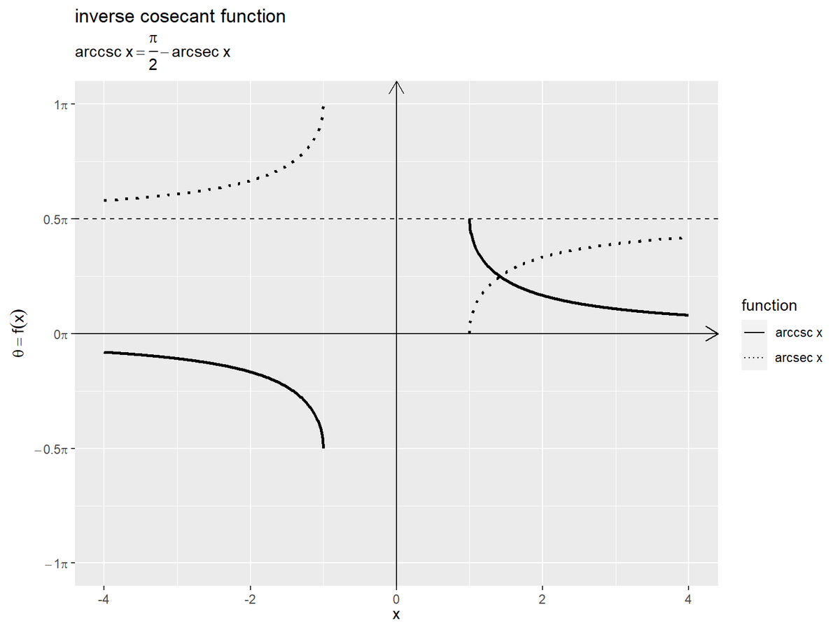
　余角の関係より、 $\mathrm{arccsc}\ x = \frac{\pi}{2} - \mathrm{arcsec}\ x$ が成り立ちます。

単位円と関数の関係

　次は、単位円における偏角(単位円上の点)と円関数(csc・sin・cos・cot)と逆円関数(arcsec)の関係を確認します。
　各関数についてはそれぞれの記事を参照してください。

グラフの作成

　変数を固定して、単位円におけるcot関数の線分とarccot関数の円弧のグラフを作成します。

・作図コード(クリックで展開)

　円関数の変数を指定して、逆円関数を計算します。

# 点用のラジアンを指定
theta <- 5/6 * pi

# 終域内のラジアンに変換
tau <- asin(sin(theta))
tau / pi

[1] 0.1666667

　csc関数の変数 $\theta$ を指定して、csc関数 $z = \csc \theta$ を変数としてarccsc関数 $\tau = \mathrm{arccsc}\ z$ を計算します。 $\tau = \arcsin(\sin \theta)$ で計算できます。
　 $\theta = 0$ の場合、 $\sin 0 = 0$ なので 1/sin(theta) が Inf になります。 $\theta = 0$ 以外( $\theta = 2 \pi$ など)の場合はプログラム上の誤差のため sin(theta) が 0 になりません。ggplot2による作図では、Inf は描画領域の端を表すため意図しないグラフになることがあります。

　円周上の点の描画用のデータフレームを作成します。

# 円周上の点の座標を作成
point_df <- tibble::tibble(
  angle = c("theta", "tau"), # 角度カテゴリ
  t = c(theta, tau), 
  x = cos(t), 
  y = sin(t), 
  point_type = c("main", "sub") # 入出力用
)
point_df

# A tibble: 2 × 5
  angle     t      x     y point_type
  <chr> <dbl>  <dbl> <dbl> <chr>     
1 theta 2.62  -0.866   0.5 main      
2 tau   0.524  0.866   0.5 sub

　円関数の入力 $\theta$ と逆円関数の出力 $\tau$ それぞれについて、単位円上の点の座標 $(x, y) = (\cos t, \sin t)$ を計算します。

　単位円の描画用のデータフレームを作成します。

# 単位円の座標を作成
circle_df <- tibble::tibble(
  t = seq(from = 0, to = 2*pi, length.out = 361), # 1周期分のラジアン
  r = 1, # 半径
  x = r * cos(t), 
  y = r * sin(t)
)

# 範囲πにおける目盛数を指定
tick_num <- 6

# 角度目盛の座標を作成
rad_tick_df <- tibble::tibble(
  i = seq(from = 0, to = 2*tick_num-0.5, by = 0.5), # 目盛番号
  t = i/tick_num * pi, # ラジアン
  r = 1, # 半径
  x = r * cos(t), 
  y = r * sin(t), 
  major_flag = i%%1 == 0, # 主・補助フラグ
  grid       = dplyr::if_else(major_flag, true = "major", false = "minor") # 目盛カテゴリ
)

　円周と角度軸目盛の座標を作成します。

　偏角の描画用のデータフレームを作成します。

# 半径線の終点の座標を作成
radius_df <- dplyr::bind_rows(
  # 始線
  tibble::tibble(
    x = 1, 
    y = 0, 
    w         = "normal", # 補助線用
    line_type = "main" # 入出力用
  ), 
  # 動径
  point_df |> 
    dplyr::select(x, y, line_type = point_type) |> 
    dplyr::mutate(
      w = dplyr::case_match(
        line_type, 
        "main" ~ "normal", 
        "sub"  ~ "thin"
      ), # 補助線用
    ), 
  # 補助線
  tibble::tibble(
    x = 0, 
    y = 1, 
    w         = "thin", # 補助線用
    line_type = "main" # 入出力用
  )
)

# 角マークの座標を作成
d_in  <- 0.2
d_spi <- 0.005
d_out <- 0.3
angle_mark_df <- dplyr::bind_rows(
  # 元の関数の入力
  tibble::tibble(
    angle = "theta", # 角度カテゴリ
    u = seq(from = 0, to = theta, length.out = 600), 
    x = (d_in + d_spi*u) * cos(u), 
    y = (d_in + d_spi*u) * sin(u)
  ), 
  # 逆関数の出力
  tibble::tibble(
    angle = "tau", # 角度カテゴリ
    u = seq(from = 0, to = tau, length.out = 600), 
    x = d_out * cos(u), 
    y = d_out * sin(u)
  )
)

# 角ラベルの座標を作成
d_in  <- 0.1
d_out <- 0.4
angle_label_df <- tibble::tibble(
  u = 0.5 * c(theta, tau), 
  x = c(d_in, d_out) * cos(u), 
  y = c(d_in, d_out) * sin(u), 
  angle_label = c("theta", "tau")
)

　 $\theta, \tau$ それぞれについて、始線と動径、角マークと角ラベルの座標を作成します。また、csc関数を示す線分用に、半径と同じ長さの補助線の座標も格納します。

　逆円関数を示す円弧の描画用のデータフレームを作成します。

# 関数円弧の座標を作成
radian_df <- tibble::tibble(
  u = seq(from = 0, to = tau, length.out = 600), 
  r = 1, # 半径
  x = r * cos(u), 
  y = r * sin(u)
)
radian_df

# A tibble: 600 × 4
          u     r     x        y
      <dbl> <dbl> <dbl>    <dbl>
 1 0            1  1    0       
 2 0.000874     1  1.00 0.000874
 3 0.00175      1  1.00 0.00175 
 4 0.00262      1  1.00 0.00262 
 5 0.00350      1  1.00 0.00350 
 6 0.00437      1  1.00 0.00437 
 7 0.00524      1  1.00 0.00524 
 8 0.00612      1  1.00 0.00612 
 9 0.00699      1  1.00 0.00699 
10 0.00787      1  1.00 0.00787 
# ℹ 590 more rows

　ラジアン $0 \leq u \leq \tau$ を作成して、単位円の円周上の(半径が $r = 1$ の)円弧の座標 $(x, y) = (\cos u, \sin u)$ を計算します。

　円関数を示す線分の描画用のデータフレームを作成します。

# 関数の描画順を指定
fnc_level_vec <- c("arccsc", "csc", "sin", "cos", "cot")

# 符号の反転フラグを設定
rev_flag <- cos(theta) < 0

# 関数線分の座標を格納
fnc_seg_df <- tibble::tibble(
  fnc = c(
    "csc", "csc", 
    "sin", 
    "cos", 
    "cot", "cot"
  ) |> 
    factor(levels = fnc_level_vec), # 関数カテゴリ
  x_from = c(
    0, ifelse(test = rev_flag, yes = 0, no = NA), 
    cos(theta), 
    0, 
    0, ifelse(test = rev_flag, yes = 0, no = NA)
  ), 
  y_from = c(
    0, ifelse(test = rev_flag, yes = 0, no = NA), 
    0, 
    0, 
    1, ifelse(test = rev_flag, yes = 1, no = NA)
  ), 
  x_to = c(
    ifelse(test = rev_flag, yes = -1/tan(theta), no = 1/tan(theta)), ifelse(test = rev_flag, yes = 1/tan(theta), no = NA), 
    cos(theta), 
    cos(theta), 
    1/tan(theta), ifelse(test = rev_flag, yes = -1/tan(theta), no = NA)
  ), 
  y_to = c(
    1, ifelse(test = rev_flag, yes = 1, no = NA), 
    sin(theta), 
    0, 
    1, ifelse(test = rev_flag, yes = 1, no = NA)
  ), 
  line_type = c(
    "main", "sub", 
    "main", 
    "main", 
    "main", "sub"
  ) # 符号の反転用
)
fnc_seg_df

# A tibble: 6 × 6
  fnc   x_from y_from   x_to  y_to line_type
  <fct>  <dbl>  <dbl>  <dbl> <dbl> <chr>    
1 csc    0          0  1.73    1   main     
2 csc    0          0 -1.73    1   sub      
3 sin   -0.866      0 -0.866   0.5 main     
4 cos    0          0 -0.866   0   main     
5 cot    0          1 -1.73    1   main     
6 cot    0          1  1.73    1   sub

　各線分に対応する関数カテゴリを fnc 列として線の描き分けなどに使います。線分の描画順(重なり順や色付け順)を因子レベルで設定します。
　各線分の始点の座標を x_from, y_from 列、終点の座標を x_to, y_to 列として、完成図を見ながら頑張って格納します。

　関数ラベルの描画用のデータフレームを作成します。

# 関数ラベルの座標を作成
fnc_label_df <- tibble::tibble(
  fnc = c(
    "arccsc", 
    "csc", "csc", 
    "sin", 
    "cos", 
    "cot", "cot"
  ) |> 
    factor(levels = fnc_level_vec), # 関数カテゴリ
  x = c(
    cos(0.5 * tau), 
    0.5 / ifelse(test = rev_flag, yes = -tan(theta), no = tan(theta)), ifelse(test = rev_flag, yes = 0.5/tan(theta), no = NA), 
    cos(theta), 
    0.5 * cos(theta), 
    0.5 / tan(theta), ifelse(test = rev_flag, yes = -0.5/tan(theta), no = NA)
  ), 
  y = c(
    sin(0.5 * tau), 
    0.5, ifelse(test = rev_flag, yes = 0.5, no = NA), 
    0.5 * sin(theta), 
    0, 
    1, ifelse(test = rev_flag, yes = 1, no = NA)
  ), 
  fnc_label = c(
    "arccsc(csc~theta)", 
    "csc~theta", "-csc~theta", 
    "sin~theta", 
    "cos~theta", 
    "cot~theta", "-cot~theta"
  ), 
  a = c(
    0, 
    0, 0, 
    90, 
    0, 
    0, 0
  ), 
  h = c(
    -0.1, 
    1.2, -0.2, 
    0.5, 
    0.5, 
    0.5, 0.5
  ), 
  v = c(
    0.5, 
    0.5, 0.5, 
    -0.5, 
    1, 
    -0.5, -0.5
  )
)
fnc_label_df

# A tibble: 7 × 7
  fnc         x     y fnc_label             a     h     v
  <fct>   <dbl> <dbl> <chr>             <dbl> <dbl> <dbl>
1 arccsc  0.966 0.259 arccsc(csc~theta)     0  -0.1   0.5
2 csc     0.866 0.5   csc~theta             0   1.2   0.5
3 csc    -0.866 0.5   -csc~theta            0  -0.2   0.5
4 sin    -0.866 0.25  sin~theta            90   0.5  -0.5
5 cos    -0.433 0     cos~theta             0   0.5   1  
6 cot    -0.866 1     cot~theta             0   0.5  -0.5
7 cot     0.866 1     -cot~theta            0   0.5  -0.5

　関数ごとに1つの線分の中点に関数名を表示することにします。
　ラベルの表示角度を a 列、表示角度に応じた左右の表示位置を h 列、上下の表示位置を v 列として指定します。

　単位円におけるarccsc関数のグラフを作成します。

# ラベル用の文字列を作成
var_label <- paste0(
  "list(", 
  "r == 1, ", 
  "theta == ", round(theta/pi, digits = 2), " * pi, ", 
  "tau == ", round(tau/pi, digits = 2), " * pi", 
  ")"
)
fnc_label_vec <- paste(
  c("arccsc(csc~theta)", "csc~theta", "sin~theta", "cos~theta", "cot~theta"), 
  c(tau, 1/sin(theta), sin(theta), cos(theta), 1/tan(theta)) |> 
    round(digits = 2), 
  sep = " == "
)

# グラフサイズの下限値・上限値を指定
axis_lower <- 1.5
axis_upper <- 3

# グラフサイズを設定
axis_x_size <- max(axis_lower, abs(1/tan(theta))) |> min(axis_upper)
axis_y_size <- 1.5

# 単位円における関数線分を作図
ggplot() + 
  geom_segment(data = rad_tick_df, 
               mapping = aes(x = 0, y = 0, xend = x, yend = y, linewidth = grid), 
               color = "white", show.legend = FALSE) + # θ軸目盛線
  geom_segment(mapping = aes(x = c(-Inf, 0), y = c(0, -Inf), 
                             xend = c(Inf, 0), yend = c(0, Inf)),
               arrow = arrow(length = unit(10, units = "pt"), ends = "last")) + # x・y軸線
  geom_path(data = circle_df, 
            mapping = aes(x = x, y = y), 
            linewidth = 1) + # 円周
  geom_segment(data = radius_df, 
               mapping = aes(x = 0, y = 0, xend = x, yend = y, 
                             linewidth = w, linetype = line_type), 
               show.legend = FALSE) + # 半径線
  geom_path(data = angle_mark_df, 
            mapping = aes(x = x, y = y, group = angle)) + # 角マーク
  geom_text(data = angle_label_df, 
            mapping = aes(x = x, y = y, label = angle_label), 
            parse = TRUE, size = 5) + # 角ラベル
  geom_text(mapping = aes(x = 0.5*cos(theta+0.1), y = 0.5*sin(theta+0.1)), 
            label = "r", parse = TRUE, 
            size = 5) + # 半径ラベル:(θ + αで表示位置を調整)
  geom_point(data = point_df, 
             mapping = aes(x = x, y = y, shape = point_type), 
             size = 4, show.legend = FALSE) + # 円周上の点
  geom_segment(mapping = aes(x = cos(theta), y = sin(theta), 
                             xend = cos(tau), yend = sin(tau)), 
               linetype = "dotted") + # 動径間の補助線
  geom_hline(yintercept = 1, linetype = "dashed") + # 補助線
  geom_path(data = radian_df, 
            mapping = aes(x = x, y = y), 
            color = "red", linewidth = 1) + # 関数円弧
  geom_segment(data = fnc_seg_df, 
               mapping = aes(x = x_from, y = y_from, xend = x_to, yend = y_to, 
                             color = fnc, linetype = line_type), 
               linewidth = 1) + # 関数線分
  geom_text(data = fnc_label_df,
            mapping = aes(x = x, y = y, label = fnc_label, color = fnc,
                          angle = a, hjust = h, vjust = v),
            parse = TRUE, show.legend = FALSE) + # 関数ラベル
  scale_color_manual(breaks = fnc_level_vec, 
                     values = c("red", scales::hue_pal()(n = length(fnc_level_vec)-1)), 
                     labels = parse(text = fnc_label_vec), name = "function") + # 凡例表示用, 色の共通化用
  scale_shape_manual(breaks = c("main", "sub"), 
                     values = c("circle", "circle open")) + # 入出力用
  scale_linetype_manual(breaks = c("main", "sub"), 
                        values = c("solid", "dashed")) + # 補助線用
  scale_linewidth_manual(breaks = c("bold", "normal", "thin", "major", "minor"), 
                         values = c(1.5, 1, 0.5, 0.5, 0.25)) + # 補助線用, 主・補助目盛線用
  guides(linewidth = "none", linetype = "none") + 
  theme(legend.text.align = 0) + 
  coord_fixed(ratio = 1, 
              xlim = c(-axis_x_size, axis_x_size), 
              ylim = c(-axis_y_size, axis_y_size)) + 
  labs(title = "circular functions", 
       subtitle = parse(text = var_label), 
       x = expression(x == r ~ cos~theta), 
       y = expression(y == r ~ sin~theta))

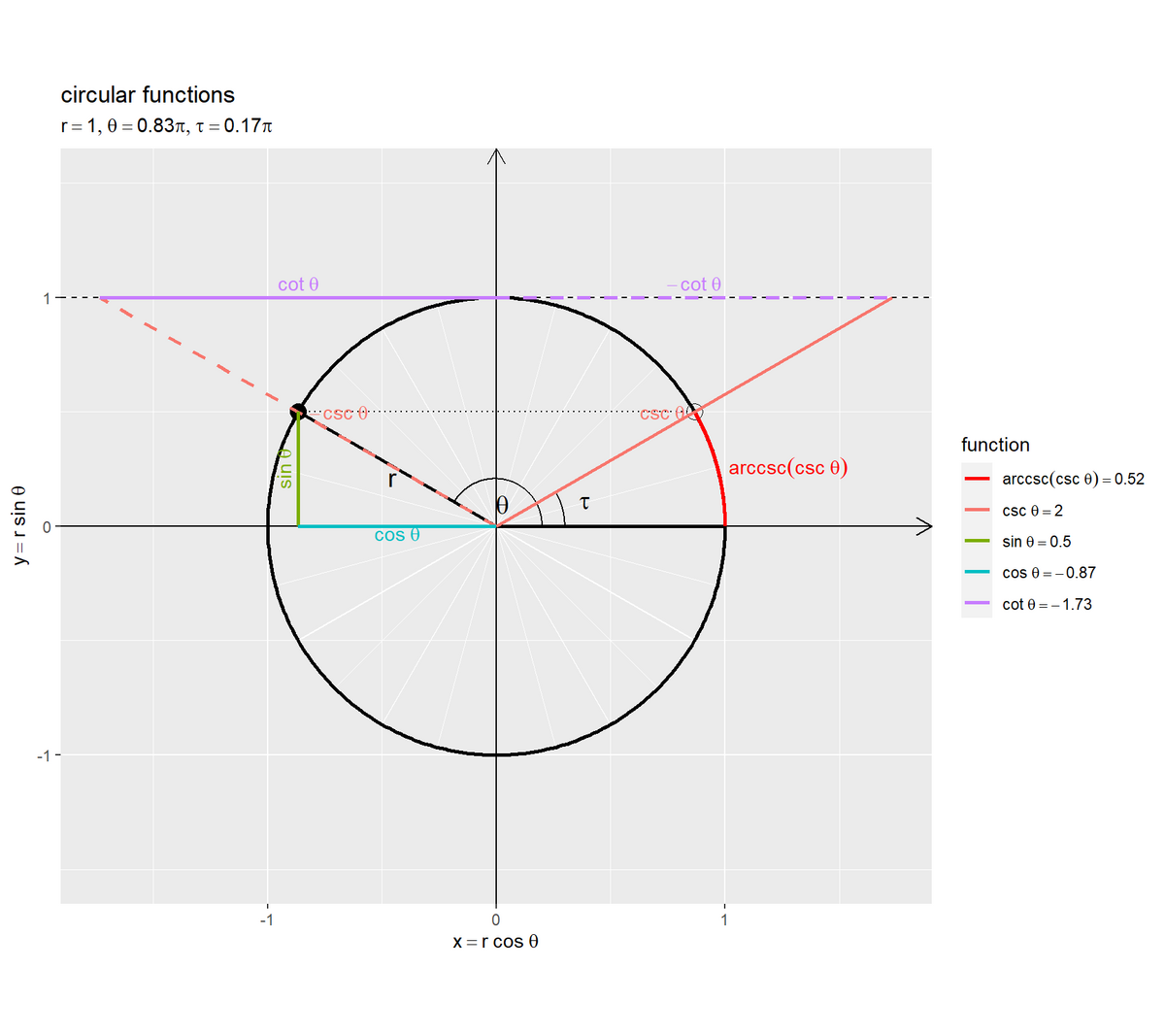
　(x座標の)符号を反転した線分を破線で示します。
　偏角(x軸の正の部分からの角度)をラジアン $\theta$ とします。中心角が $\theta$ の弧長は $l = r \theta$ です。よって(ラジアンを用いると)、単位円における( $r = 1$ のとき)偏角 $\theta$ と弧長 $l$ が一致します。半径が $r$ の円周上の点の座標は $(x, y) = (r \cos \theta, r \sin \theta)$ です。
　csc関数の値を $z = \csc \theta$ 、arccsc関数の値を $\tau = \mathrm{arccsc} z$ と置く(csc関数の入力を $\theta$ 、arccsc関数の出力を $\tau$ とする)と、csc関数が $z$ になる偏角(弧長)が $\tau$ であり、 $\csc \theta = \csc \tau$ となります。

アニメーションの作成

　変数を変化させて、単位円におけるarccsc関数のアニメーションを作成します。
　作図コードについては「GitHub - anemptyarchive/Mathematics/.../arccsc_definition.R」を参照してください。

　単位円における偏角とarccsc関数の円弧の関係を可視化します。

　csc関数の終域 $\csc \theta \leq -1\ \mathrm{or}\ 1 \leq \csc \theta$ をarccsc関数の定義域 $z \leq -1\ \mathrm{or}\ 1 \leq z$ として、終域が $-\frac{\pi}{2} \leq \mathrm{arccsc}\ z \lt 0\ \mathrm{or}\ 0 \lt \mathrm{arccsc}\ z \leq \frac{\pi}{2}$ ( $\sin 0 = 0$ なので(0除算になるので)csc関数とcot関数が定義できない $0$ を除く $-\frac{\pi}{2}$ から $\frac{\pi}{2}$ の範囲) になるのを確認できます。
　 $n$ を整数として $\theta = n \pi$ のとき、csc関数とcot関数を示す線が平行になり(半直線)になるためそれぞれ定義できません。

単位円と曲線の関係

　最後は、単位円と関数曲線のグラフを作成して、変数(ラジアン)と座標の関係を確認します。
　作図コードについては「arccsc_definition.R」を参照してください。

変数と座標の関係

　変数に応じて移動する円周上の点と曲線上の点のアニメーションを作成します。

　円周上の点とarccsc関数曲線上の点の関係を可視化します。

　 $\csc \theta$ に対応する偏角(弧長) $\tau = \mathrm{arccsc}(\csc \theta)$ と曲線の縦軸の値、 $z = \csc \theta = \csc \tau$ と曲線の横軸の値が一致するのを確認できます。

　この記事では、逆csc関数を確認しました。

おわりに

　逆円関数編のラストです！円関数編の水増し的な内容になるのではと心配していたのですが、円関数自体の理解も深まったのでやってみて良かったです。弧度法を使う嬉しさもたぶん分かりました。
　最後にですが、このブログでは三角関数のことを円関数と呼びます。円周率を6.28...にしたい気持ちもほんの少し分かった気がします。

【次の内容】

つづく...といきたいけど次にあたるのは何でしょう。

からっぽのしょこ

読んだら書く！書いたら読む！同じ事は二度調べ(たく)ない

【R】arccsc関数の定義の可視化

はじめに

arccsc関数の定義の可視化

定義式の確認

arccsc関数とcsc関数の関係

arccsc関数とarcsin関数の関係

逆数によるarcsin関数

逆数によるarccsc関数

曲線の形状

曲線の作成

単位円と関数の関係

グラフの作成

アニメーションの作成

単位円と曲線の関係

変数と座標の関係

おわりに