はじめに

　円関数(三角関数)の定義や性質、公式などを可視化して理解しようシリーズです。

　この記事では、R言語でcotangent関数のグラフを作成します。

【前の内容】

t.co

【他の記事一覧】

www.anarchive-beta.com

【この記事の内容】

はじめに
cot関数の定義の可視化
参考書籍
おわりに

cot関数の定義の可視化

　cot関数(余接関数・コタンジェント関数・cotangent function)の定義をグラフで確認します。cot関数は、円関数(circular functions)・三角関数(trigonometric functions)の1つです。
　cot関数の形状(振幅・周期・位相・切片)の変化については各パラメータの記事や「cot関数の波形の可視化」を参照してください。

　利用するパッケージを読み込みます。

# 利用パッケージ
library(tidyverse)

　この記事では、基本的に パッケージ名::関数名() の記法を使うので、パッケージの読み込みは不要です。ただし、作図コードについてはパッケージ名を省略するので、ggplot2 を読み込む必要があります。
　また、ネイティブパイプ演算子 |> を使います。magrittr パッケージのパイプ演算子 %>% に置き換えられますが、その場合は magrittr を読み込む必要があります。

定義式の確認

　まずは、cot関数の定義式を確認します。
　tan関数については「【R】tan関数の定義の可視化 - からっぽのしょこ」を参照してください。

　cot関数は、tan関数の逆数(cos関数とsin関数の商)で定義されます。

$\displaystyle \cot x = \frac{1}{\tan x} = \frac{\cos x}{\sin x}$

　ただし、 $n$ を正負の整数として $x = n \pi$ のとき、 $\sin x = 0$ であり、0除算になるため定義できません。変数 $x$ はラジアン(弧度法の角度)、 $\pi$ は円周率です。

曲線の形状

　続いて、cot関数の曲線のグラフを作成します。

曲線の作成

・作図コード(クリックで展開)

　変数の範囲を指定して、座標計算用のベクトルを作成します。

# 変数(ラジアン)の範囲を指定
theta_vec <- seq(from = -2*pi, to = 2*pi, length.out = 1001)
head(theta_vec)

[1] -6.283185 -6.270619 -6.258053 -6.245486 -6.232920 -6.220353

　変数(ラジアン) $\theta$ の範囲を指定して、数値ベクトルを作成します。範囲を $\pi$ の倍数にすると周期性を確認しやすくなります。円周率 $\pi$ は pi で扱えます。

　曲線の描画用のデータフレームを作成します。

# 閾値を指定
threshold <- 4

# 曲線の座標を作成
curve_df <- tibble::tibble(
  t     = theta_vec, 
  cot_t = 1/tan(t), 
  tan_t = tan(t), 
  sin_t = sin(t), 
  cos_t = cos(t)
) |> 
  dplyr::mutate(
    cot_t = dplyr::if_else(
      (cot_t >= -threshold & cot_t <= threshold), true = cot_t, false = NA_real_
    ), 
    tan_t = dplyr::if_else(
      (tan_t >= -threshold & tan_t <= threshold), true = tan_t, false = NA_real_
    )
  ) # 閾値外を欠損値に置換
curve_df

# A tibble: 1,001 × 5
       t cot_t    tan_t    sin_t cos_t
   <dbl> <dbl>    <dbl>    <dbl> <dbl>
 1 -6.28    NA 2.45e-16 2.45e-16 1    
 2 -6.27    NA 1.26e- 2 1.26e- 2 1.00 
 3 -6.26    NA 2.51e- 2 2.51e- 2 1.00 
 4 -6.25    NA 3.77e- 2 3.77e- 2 0.999
 5 -6.23    NA 5.03e- 2 5.02e- 2 0.999
 6 -6.22    NA 6.29e- 2 6.28e- 2 0.998
 7 -6.21    NA 7.55e- 2 7.53e- 2 0.997
 8 -6.20    NA 8.82e- 2 8.79e- 2 0.996
 9 -6.18    NA 1.01e- 1 1.00e- 1 0.995
10 -6.17    NA 1.14e- 1 1.13e- 1 0.994
# ℹ 991 more rows

　変数 $\theta$ と関数 $\cot \theta$ の値をデータフレームに格納します。比較用に、 $\tan \theta, \sin \theta, \cos \theta$ の値も格納しておきます。tan関数は tan()、sin関数は sin()、cos関数は cos() で、cot関数は tan() を使って計算できます。
　ただし範囲によっては、 $\cot \theta, \tan \theta$ が発散するので、閾値 threshold を指定しておき、閾値外の値を(数値型の)欠損値 NA に置き換えます。

　ラジアン軸目盛の表示用のベクトルを作成します。装飾用の処理です。

# 半周期(範囲π)における目盛数(分母の値)を指定
tick_num <- 2

# 目盛番号(分子の値)の範囲を設定
tick_min <- floor(min(theta_vec) / pi) * tick_num
tick_max <- ceiling(max(theta_vec) / pi) * tick_num

# 目盛番号(分子の値)を作成
tick_vec <- tick_min:tick_max

# 目盛位置を作成
rad_break_vec <- tick_vec/tick_num * pi

# 目盛ラベルを作成
rad_label_vec <- paste(round(rad_break_vec/pi, digits = 2), "* pi")
head(tick_vec); head(rad_break_vec); head(rad_label_vec)

[1] -4 -3 -2 -1  0  1
[1] -6.283185 -4.712389 -3.141593 -1.570796  0.000000  1.570796
[1] "-2 * pi"   "-1.5 * pi" "-1 * pi"   "-0.5 * pi" "0 * pi"    "0.5 * pi"

　ラジアン $\theta$ に関する軸目盛ラベルを $\frac{i}{n} \pi$ を小数にした形で表示することにします。 $n$ は半周期( $\pi$ 間隔の範囲)における目盛数、 $i$ は(負の数を含む)目盛番号に対応します。
　theta_vec の最小値・最大値に対して、 $\theta = \frac{i}{n} \pi$ を $i$ について整理した $i = \frac{\theta}{\pi} n$ を計算して、最小番号から最大番号までの整数を作成します。整数にするために、小数部分に関して最小値は floor() で切り捨て、最大値は ceiling() で切り上げておきます。
　作成した目盛番号に対応する目盛位置(ラジアン)を $\theta = \frac{i}{n} \pi$ で計算します。

　ラベルとして数式(ギリシャ文字や記号)を表示する場合は、expression() の記法を用います。その際に、オブジェクト(プログラム上の変数)を使う場合は、文字列として作成しておき parse() の text 引数に渡します。

　漸近線の描画用のベクトルを作成します。

# 漸近線の範囲を設定:(π単位で切り捨て・切り上げ)
theta_lower <- floor(min(theta_vec) / pi) * pi
theta_upper <- ceiling(max(theta_vec) / pi) * pi

# 漸近線の位置を作成
asymptote_break_vec <- seq(from = theta_lower, to = theta_upper, by = pi)

# 漸近線のラベルを作成
asymptote_label_vec <- paste(round(asymptote_break_vec/pi, digits = 2), "* pi")
head(asymptote_break_vec); head(asymptote_label_vec)

[1] -6.283185 -3.141593  0.000000  3.141593  6.283185
[1] "-2 * pi" "-1 * pi" "0 * pi"  "1 * pi"  "2 * pi"

　 $\cot \theta$ が発散する位置に漸近線と目盛ラベルを表示することにします。
　ラジアン軸目盛と同様に、theta_vec の最小値・最大値を用いて、ラジアン $\theta = n \pi$ ( $n$ は整数)とラベルを作成します。

　cot関数(とtan関数)のグラフを作成します。

# ラベル用の文字列を作成
def_label <- paste0(
  "paste(", 
  "cot~theta == frac(1, tan~theta), ", 
  "{} == frac(cos~theta, sin~theta)", 
  ")"
)

# 関数曲線を作図
ggplot() + 
  geom_segment(mapping = aes(x = c(-Inf, 0), y = c(0, -Inf), 
                             xend = c(Inf, 0), yend = c(0, Inf)), 
               arrow = arrow(length = unit(10, units = "pt"), ends = "last")) + # x・y軸線
  geom_vline(xintercept = asymptote_break_vec, 
             linetype = "twodash") + # 漸近線
  geom_line(data = curve_df, 
            mapping = aes(x = t, y = cot_t, linetype = "cot"), 
            linewidth = 1, na.rm = TRUE) + # cot曲線
  geom_line(data = curve_df, 
            mapping = aes(x = t, y = tan_t, linetype = "tan"), 
            linewidth = 1, na.rm = TRUE) + # tan曲線
  scale_linetype_manual(breaks = c("cot", "tan"), 
                        values = c("solid", "dotted"), 
                        labels = c(expression(cot~theta), expression(tan~theta)), 
                        name = "function") + # 凡例表示用
  scale_x_continuous(breaks = rad_break_vec, 
                     labels = parse(text = rad_label_vec), 
                     sec.axis = sec_axis(trans = ~., 
                                         breaks = asymptote_break_vec, 
                                         labels = parse(text = asymptote_label_vec), 
                                         name = "asymptote")) + # ラジアン軸目盛
  guides(linetype = guide_legend(override.aes = list(linewidth = 0.5))) + # 凡例の体裁
  theme(legend.text.align = 1) + # 図の体裁
  coord_fixed(ratio = 1) + # アスペクト比
  labs(title = "cotangent function", 
       subtitle = parse(text = def_label), 
       x = expression(theta), 
       y = expression(f(theta)))

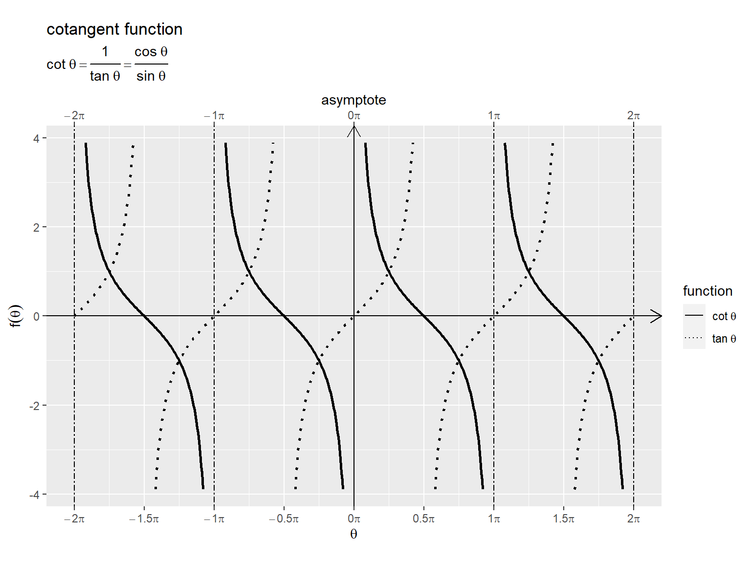
　cot曲線を実線、tan曲線を点線で、また漸近線を鎖線で示します。
　横軸(変数) $\theta$ はラジアン(弧度法の角度)、 $\pi$ は円周率です。

　 $n$ を整数として、 $\theta$ 軸が $n \pi$ の点( $0$ を中心に $\pi$ 間隔)で、 $\tan \theta = 0$ であり $\cot \theta$ が発散するのを確認できます。
　余角の関係より、 $\cot \theta = \tan(\frac{\pi}{2} - \theta)$ が成り立ちます。

・作図コード(クリックで展開)

　cot関数(とsin関数・cos関数)のグラフを作成します。

# 関数曲線を作図
ggplot() + 
  geom_segment(mapping = aes(x = c(-Inf, 0), y = c(0, -Inf), 
                             xend = c(Inf, 0), yend = c(0, Inf)), 
               arrow = arrow(length = unit(10, units = "pt"), ends = "last")) + # x・y軸線
  geom_vline(xintercept = asymptote_break_vec, 
             linetype = "twodash") + # 漸近線
  geom_line(data = curve_df, 
            mapping = aes(x = t, y = cot_t, linetype = "cot"), 
            linewidth = 1, na.rm = TRUE) + # cot曲線
  geom_line(data = curve_df, 
            mapping = aes(x = t, y = sin_t, linetype = "sin"), 
            linewidth = 1) + # sin曲線
  geom_line(data = curve_df, 
            mapping = aes(x = t, y = cos_t, linetype = "cos"), 
            linewidth = 1) + # cos曲線
  scale_linetype_manual(breaks = c("cot", "sin", "cos"), 
                        values = c("solid", "dashed", "dotted"), 
                        labels = c(expression(cot~theta), expression(sin~theta), expression(cos~theta)), 
                        name = "function") + # 凡例表示用
  scale_x_continuous(breaks = rad_break_vec, 
                     labels = parse(text = rad_label_vec), 
                     sec.axis = sec_axis(trans = ~., 
                                         breaks = asymptote_break_vec, 
                                         labels = parse(text = asymptote_label_vec), 
                                         name = "asymptote")) + # ラジアン軸目盛
  guides(linetype = guide_legend(override.aes = list(linewidth = 0.5))) + # 凡例の体裁
  theme(legend.text.align = 1) + # 図の体裁
  coord_fixed(ratio = 1) + # アスペクト比
  labs(title = "cotangent function", 
       subtitle = parse(text = def_label), 
       x = expression(theta), 
       y = expression(f(theta)))

　cot曲線を実線、sin曲線を破線、cos曲線を点線で示します。

　 $\theta$ 軸が $n \pi$ の点で、 $\sin \theta = 0$ であり $\cot \theta$ が発散するのを確認できます。また、 $\theta$ 軸が $(\frac{1}{2} + n) \pi$ の点( $\frac{1}{2} \pi$ を中心に $\pi$ 間隔)で、 $\cos \theta = 0$ であり $\cot \theta = 0$ になります。

　次からは、単位円との関係を見ていきます。

単位円の作成

　円関数の可視化に利用する単位円(unit circle)のグラフを確認します。
　円の作図や度数法と弧度法(角度とラジアン)の関係については「【R】黄金角の定義の可視化 - からっぽのしょこ」を参照してください。

・作図コード(クリックで展開)

　単位円の描画用のデータフレームを作成します。

# 円周の座標を作成
circle_df <- tibble::tibble(
  t = seq(from = 0, to = 2*pi, length.out = 361), # 1周期分のラジアン
  r = 1, # 半径
  x = r * cos(t), 
  y = r * sin(t)
)
circle_df

# A tibble: 361 × 4
        t     r     x      y
    <dbl> <dbl> <dbl>  <dbl>
 1 0          1 1     0     
 2 0.0175     1 1.00  0.0175
 3 0.0349     1 0.999 0.0349
 4 0.0524     1 0.999 0.0523
 5 0.0698     1 0.998 0.0698
 6 0.0873     1 0.996 0.0872
 7 0.105      1 0.995 0.105 
 8 0.122      1 0.993 0.122 
 9 0.140      1 0.990 0.139 
10 0.157      1 0.988 0.156 
# ℹ 351 more rows

　1周分のラジアン $0 \leq \theta \leq 2 \pi$ を作成して、単位円の円周のx座標 $x = \cos \theta$ とy座標 $y = \sin \theta$ を計算します。

　角度(ラジアン)目盛の描画用のデータフレームを作成します。

# 半円(範囲π)における目盛数(分母の値)を指定
tick_num <- 6

# 角度目盛の座標を作成:(補助目盛有り)
d <- 1.1
rad_tick_df <- tibble::tibble(
  # 座標用
  i     = seq(from = 0, to = 2*tick_num-0.5, by = 0.5), # 目盛番号(分子の値)
  t_deg = i/tick_num * 180, # 度数法の角度
  t_rad = i/tick_num * pi,  # 弧度法の角度(ラジアン)
  r     = 1, # 半径
  x     = r * cos(t_rad), 
  y     = r * sin(t_rad), 
  major_flag = i%%1 == 0, # 主・補助フラグ
  grid       = dplyr::if_else(major_flag, true = "major", false = "minor"), # 目盛カテゴリ
  # ラベル用
  deg_label  = dplyr::if_else(
    major_flag, true = paste0(round(t_deg, digits = 1), "*degree"), false = ""
  ), # 角度ラベル
  rad_label  = dplyr::if_else(
    major_flag, true = paste0("frac(", i, ", ", tick_num, ") ~ pi"), false = ""
  ), # ラジアンラベル
  label_x = d * x, 
  label_y = d * y, 
  a = t_deg + 90, 
  h = 1 - (x * 0.5 + 0.5), 
  v = 1 - (y * 0.5 + 0.5), 
  tick_mark = dplyr::if_else(major_flag, true = "|", false = "") # 目盛指示線用
)
rad_tick_df

# A tibble: 24 × 16
       i t_deg t_rad     r         x     y major_flag grid  deg_label  rad_label
   <dbl> <dbl> <dbl> <dbl>     <dbl> <dbl> <lgl>      <chr> <chr>      <chr>    
 1   0       0 0         1  1   e+ 0 0     TRUE       major "0*degree" "frac(0,…
 2   0.5    15 0.262     1  9.66e- 1 0.259 FALSE      minor ""         ""       
 3   1      30 0.524     1  8.66e- 1 0.5   TRUE       major "30*degre… "frac(1,…
 4   1.5    45 0.785     1  7.07e- 1 0.707 FALSE      minor ""         ""       
 5   2      60 1.05      1  5   e- 1 0.866 TRUE       major "60*degre… "frac(2,…
 6   2.5    75 1.31      1  2.59e- 1 0.966 FALSE      minor ""         ""       
 7   3      90 1.57      1  6.12e-17 1     TRUE       major "90*degre… "frac(3,…
 8   3.5   105 1.83      1 -2.59e- 1 0.966 FALSE      minor ""         ""       
 9   4     120 2.09      1 -5   e- 1 0.866 TRUE       major "120*degr… "frac(4,…
10   4.5   135 2.36      1 -7.07e- 1 0.707 FALSE      minor ""         ""       
# ℹ 14 more rows
# ℹ 6 more variables: label_x <dbl>, label_y <dbl>, a <dbl>, h <dbl>, v <dbl>,
#   tick_mark <chr>

　「曲線の作図」のときと同様に、目盛番号と対応するラジアンを作成して、円周上の座標とラベル用の文字列を作成します。ただし、補助目盛も作成します。主目盛と補助目盛を major_flag 列または grid 列で描き分けます。
　目盛ラベル用の座標を label_x, label_y 列として、表示位置を原点からのノルム(半径) d で調整します。

　単位円と角度目盛のグラフを作成します。

# グラフサイズを設定
axis_size <- 1.5

# 単位円を作図
ggplot() + 
  geom_segment(data = rad_tick_df, 
               mapping = aes(x = 0, y = 0, xend = x, yend = y), 
               linetype = "dotted") + # 角度目盛線
  geom_text(data = rad_tick_df, 
            mapping = aes(x = x, y = y, angle = a, label = tick_mark), 
            size = 2) + # 角度目盛指示線
  geom_text(data = rad_tick_df, 
            mapping = aes(x = label_x, y = label_y, label = deg_label, hjust = h, vjust = v), 
            parse = TRUE) + # 角度目盛ラベル
  geom_path(data = circle_df, 
            mapping = aes(x = x, y = y), 
            linewidth = 1) + # 円周
  coord_fixed(ratio = 1, 
              xlim = c(-axis_size, axis_size), 
              ylim = c(-axis_size, axis_size)) + # アスペクト比
  labs(title = "unit circle", 
       subtitle = expression(r == 1), 
       x = expression(x == r ~ cos~theta), 
       y = expression(y == r ~ sin~theta))

　原点を中心とする半径 $r$ の円周の座標は $(x, y) = (r \cos \theta, r \sin \theta)$ です。半径が $r = 1$ の円を単位円と呼びます。(半径や開始位置に関わらず)偏角が $2 \pi$ (度数法だと $360^{\circ}$ )で1周します。
　度数法の角度 $\theta^{\circ}$ と弧度法の角度 $\theta$ は $\theta = \frac{2 \pi}{360^{\circ}} \theta^{\circ}$ の関係です。

　このグラフ上に円関数の値を線分として描画します。

単位円と関数の関係

　次は、単位円における偏角(単位円周上の点)と円関数(cot・tan・sin・cos・exsec・excsc)の関係を可視化します。
　各関数についてはそれぞれの記事を参照してください。

グラフの作成

　変数を固定して、単位円におけるcot関数のグラフを作成します。

・作図コード(クリックで展開)

　変数を指定して、円周上の点の描画用のデータフレームを作成します。

# 点用のラジアンを指定
theta <- 1/6 * pi

# 円周上の点の座標を作成
point_df <- tibble::tibble(
  t = theta, 
  x = cos(t), 
  y = sin(t)
)
point_df

# A tibble: 1 × 3
      t     x     y
  <dbl> <dbl> <dbl>
1 0.524 0.866   0.5

　変数 $\theta$ を指定して、単位円の円周上の点の座標 $(x, y) = (\cos \theta, \sin \theta)$ を計算します。
　 $\theta = 0$ の場合、 $\tan 0 = 0$ なので 1/tan(theta) が Inf になります。 $\theta = 0$ 以外( $\theta = 2 \pi$ など)の場合はプログラム上の誤差のため tan(theta) が 0 になりません。ggplot2による作図では、Inf は描画領域の端を表すため意図しないグラフになることがあります。変数に微小な値を加えるなどして回避できます。

　角マークの描画用のデータフレームを作成します。

# 角マークの座標を作成
d  <- 0.2
ds <- 0.005
angle_mark_df <- tibble::tibble(
  u = seq(from = 0, to = theta, length.out = 600), 
  x = (d + ds*u) * cos(u), 
  y = (d + ds*u) * sin(u)
)
angle_mark_df

# A tibble: 600 × 3
          u     x        y
      <dbl> <dbl>    <dbl>
 1 0        0.2   0       
 2 0.000874 0.200 0.000175
 3 0.00175  0.200 0.000350
 4 0.00262  0.200 0.000525
 5 0.00350  0.200 0.000699
 6 0.00437  0.200 0.000874
 7 0.00524  0.200 0.00105 
 8 0.00612  0.200 0.00122 
 9 0.00699  0.200 0.00140 
10 0.00787  0.200 0.00157 
# ℹ 590 more rows

　2つの線分のなす角(偏角) $\theta$ を示す角マークとして、 $0 \leq u \leq \theta$ のラジアンを作成して、係数が $d$ の螺旋の座標 $(x, y) = (d u \cos u, d u \sin u)$ を計算します。この例では、ノルムの基準値 d と間隔用の係数 ds でサイズを調整します。ds を 0 にすると、半径が $d$ の円弧の座標 $(x, y) = (d \cos u, d \sin u)$ になります。

　角ラベルの描画用のデータフレームを作成します。

# 角ラベルの座標を計算
d <- 0.3
angle_label_df <- tibble::tibble(
  u = 0.5 * theta, 
  x = d * cos(u), 
  y = d * sin(u)
)
angle_label_df

# A tibble: 1 × 3
      u     x      y
  <dbl> <dbl>  <dbl>
1 0.262 0.290 0.0776

　角マークの中点に角ラベルを配置することにします。 $u = \frac{\theta}{2}$ のラジアンを作成して、円弧上の点の座標を計算します。原点からのノルム d で表示位置を調整します。

　各種ラベルの表示用の文字列を作成します。

# ラベル用の文字列を作成
var_label <- paste0(
  "list(", 
  "r == 1, ", 
  "theta == ", round(theta/pi, digits = 2), " * pi", 
  ")"
)
fnc_label_vec <- paste(
  c("cot~theta", "tan~theta", "sin~theta", "cos~theta", "exsec~theta", "excsc~theta"), 
  c(1/tan(theta), tan(theta), sin(theta), cos(theta), 1/cos(theta)-1, 1/sin(theta)-1) |> 
    round(digits = 2), 
  sep = " == "
)
var_label; fnc_label_vec

[1] "list(r == 1, theta == 0.17 * pi)"
[1] "cot~theta == 1.73"   "tan~theta == 0.58"   "sin~theta == 0.5"   
[4] "cos~theta == 0.87"   "exsec~theta == 0.15" "excsc~theta == 1"

　サブタイトル用の変数ラベル、凡例用の関数ラベルを作成します。
　expression() の記法では、等号は "=="、複数の(数式上の)変数は "list(変数1, 変数2)" で並べて表示できます。

　ここまでは、共通の処理です。ここからは、2つの方法で図示します。

パターン1

　1つ目の方法では、y軸線から伸びる線分としてcot関数を可視化します。

・作図コード(クリックで展開)

　偏角を示す線分と補助線用の線分の描画用のデータフレームを作成します。

# 半径線の座標を作成
radius_df <- tibble::tibble(
  x_from = c(0, 0, 0, 1/tan(theta)), 
  y_from = c(0, 0, 0, 0), 
  x_to   = c(1, cos(theta), 0, 1/tan(theta)), 
  y_to   = c(0, sin(theta), 1, 1), 
  w      = c("normal", "normal", "thin", "thin") # 補助線用
)
radius_df

# A tibble: 4 × 5
  x_from y_from  x_to  y_to w     
   <dbl>  <dbl> <dbl> <dbl> <chr> 
1   0         0 1       0   normal
2   0         0 0.866   0.5 normal
3   0         0 0       1   thin  
4   1.73      0 1.73    1   thin

　偏角用の線分として、原点と点 $(1, 0)$ を結ぶ線分(始線)、原点と点 $(\cos \theta, \sin \theta)$ を結ぶ線分(動径)用に、原点 $(0, 0)$ と円周上の2点の座標を格納します。
　また、関数線分の補助線用の線分として、長さが1(半径と同じ)線分の座標を完成図と睨めっこして格納します。
　各線分の始点の座標を x_from, y_from 列、終点の座標を x_to, y_to 列とします。
　偏角用と補助線用の線分を、線の太さで描き分けることにします。線の太さを区別する文字列を w 列とします。文字列自体は自由です。

　関数を示す線分の描画用のデータフレームを作成します。

# 関数の描画順を指定
fnc_level_vec <- c("cot", "tan", "sin", "cos", "exsec", "excsc")

# 関数線分の座標を作成
fnc_seg_df <- tibble::tibble(
  fnc = c(
    "cot", "cot", 
    "tan", 
    "sin", "sin", 
    "cos", "cos", 
    "exsec", 
    "excsc"
  ) |> 
    factor(levels = fnc_level_vec), # 関数カテゴリ
  x_from = c(
    0, 0, 
    1, 
    0, cos(theta), 
    0, 0, 
    cos(theta), 
    cos(theta)
  ), 
  y_from = c(
    0, 1, 
    0, 
    0, 0, 
    0, sin(theta), 
    sin(theta), 
    sin(theta)
  ), 
  x_to = c(
    1/tan(theta), 1/tan(theta), 
    1, 
    0, cos(theta), 
    cos(theta), cos(theta), 
    1, 
    1/tan(theta)
  ), 
  y_to = c(
    0, 1, 
    tan(theta), 
    sin(theta), sin(theta), 
    0, sin(theta), 
    tan(theta), 
    1
  ), 
  w = c(
    "bold", "normal", 
    "normal", 
    "normal", "normal", 
    "thin", "normal", 
    "bold", 
    "thin"
  ) # 重なり対策用
)
fnc_seg_df

# A tibble: 9 × 6
  fnc   x_from y_from  x_to  y_to w     
  <fct>  <dbl>  <dbl> <dbl> <dbl> <chr> 
1 cot    0        0   1.73  0     bold  
2 cot    0        1   1.73  1     normal
3 tan    1        0   1     0.577 normal
4 sin    0        0   0     0.5   normal
5 sin    0.866    0   0.866 0.5   normal
6 cos    0        0   0.866 0     thin  
7 cos    0        0.5 0.866 0.5   normal
8 exsec  0.866    0.5 1     0.577 bold  
9 excsc  0.866    0.5 1.73  1     thin

　各線分に対応する関数カテゴリを fnc 列として線の描き分けなどに使います。線分の描画順(重なり順)や色付け順を因子レベルで設定します。
　各線分の始点の座標を x_from, y_from 列、終点の座標を x_to, y_to 列として、完成図を見ながら頑張って格納します。
　線分が重なることがあるので、線の太さで描き分けることにします。先に描画される線分を太く、後から描画される線分を細くするように、先ほどの文字列を w 列に指定します。

　関数ラベルの描画用のデータフレームを作成します。

# 関数ラベルの座標を作成
fnc_label_df <- tibble::tibble(
  fnc = c("cot", "tan", "sin", "cos", "exsec", "excsc") |> 
    factor(levels = fnc_level_vec), # 関数カテゴリ
  x = c(
    0.5 / tan(theta), 
    1, 
    0, 
    0.5 * cos(theta), 
    0.5 * (cos(theta) + 1), 
    0.5 * (cos(theta) + 1/tan(theta))
  ), 
  y = c(
    1, 
    0.5 * tan(theta), 
    0.5 * sin(theta), 
    0, 
    0.5 * (sin(theta) + tan(theta)), 
    0.5 * (sin(theta) + 1)
  ), 
  fnc_label = c("cot~theta", "tan~theta", "sin~theta", "cos~theta", "exsec~theta", "excsc~theta"), 
  a = c( 0,   90,  90,  0,   0,    0), 
  h = c( 0.5, 0.5, 0.5, 0.5, 1.1, -0.1), 
  v = c(-0.5, 1,  -0.5, 1,   0.5,  0.5)
)
fnc_label_df

# A tibble: 6 × 7
  fnc       x     y fnc_label       a     h     v
  <fct> <dbl> <dbl> <chr>       <dbl> <dbl> <dbl>
1 cot   0.866 1     cot~theta       0   0.5  -0.5
2 tan   1     0.289 tan~theta      90   0.5   1  
3 sin   0     0.25  sin~theta      90   0.5  -0.5
4 cos   0.433 0     cos~theta       0   0.5   1  
5 exsec 0.933 0.539 exsec~theta     0   1.1   0.5
6 excsc 1.30  0.75  excsc~theta     0  -0.1   0.5

　関数ごとに1つの線分の中点に関数名を表示することにします。
　ラベルの表示角度を a 列、表示角度に応じた左右の表示位置を h 列、上下の表示位置を v 列として指定します。

　単位円におけるcot関数のグラフを作成します。

# グラフサイズの下限値・上限値を指定
axis_lower <- 1.5
axis_upper <- 3

# グラフサイズを設定
axis_x_min <- min(-axis_lower, 1/tan(theta)) |> max(-axis_upper)
axis_x_max <- max(axis_lower, 1/tan(theta)) |> min(axis_upper)
axis_y_min <- min(-axis_lower, tan(theta)) |> max(-axis_upper)
axis_y_max <- max(axis_lower, tan(theta)) |> min(axis_upper)

# 単位円における関数線分を作図
ggplot() + 
  geom_segment(data = rad_tick_df, 
               mapping = aes(x = 0, y = 0, xend = x, yend = y, linewidth = grid), 
               color = "white", show.legend = FALSE) + # 角度目盛線
  geom_text(data = rad_tick_df, 
            mapping = aes(x = x, y = y, angle = a, label = tick_mark), 
            size = 2) + # 角度目盛指示線
  geom_text(data = rad_tick_df, 
            mapping = aes(x = label_x, y = label_y, label = rad_label, hjust = h, vjust = v), 
            parse = TRUE) + # 角度目盛ラベル
  geom_path(data = circle_df, 
            mapping = aes(x = x, y = y), 
            linewidth = 1) + # 円周
  geom_segment(data = radius_df, 
               mapping = aes(x = x_from, y = y_from, xend = x_to, yend = y_to, linewidth = w), 
               show.legend = FALSE) + # 半径線
  geom_path(data = angle_mark_df, 
            mapping = aes(x = x, y = y)) + # 角マーク
  geom_text(data = angle_label_df, 
            mapping = aes(x = x, y = y), 
            label = "theta", parse = TRUE, 
            size = 5) + # 角ラベル
  geom_text(mapping = aes(x = 0.5*cos(theta+0.1), y = 0.5*sin(theta+0.1)), 
            label = "r", parse = TRUE, 
            size = 5) + # 半径ラベル:(θ + αで表示位置を調整)
  geom_point(data = point_df, 
             mapping = aes(x = x, y = y), 
             size = 4) + # 円周上の点
  geom_hline(yintercept = 1, linetype = "dashed") + # 補助線
  geom_segment(data = fnc_seg_df, 
               mapping = aes(x = x_from, y = y_from, xend = x_to, yend = y_to, 
                             color = fnc, linewidth = w)) + # 関数線分
  geom_text(data = fnc_label_df, 
            mapping = aes(x = x, y = y, label = fnc_label, color = fnc, 
                          hjust = h, vjust = v, angle = a), 
            parse = TRUE, show.legend = FALSE) + # 関数ラベル
  scale_color_hue(labels = parse(text = fnc_label_vec), name = "function") + # 凡例表示用
  scale_linewidth_manual(breaks = c("bold", "normal", "thin", "major", "minor"), 
                         values = c(1.5, 1, 0.5, 0.5, 0.25)) + # 補助線用, 重なり対策用, 主・補助目盛線用
  guides(color = guide_legend(override.aes = list(linewidth = 1)), 
         linewidth = "none") + 
  theme(legend.text.align = 0) + 
  coord_fixed(ratio = 1, 
              xlim = c(axis_x_min, axis_x_max), 
              ylim = c(axis_y_min, axis_y_max)) + 
  labs(title = "circular functions", 
       subtitle = parse(text = var_label), 
       x = expression(x == r ~ cos~theta), 
       y = expression(y == r ~ sin~theta))

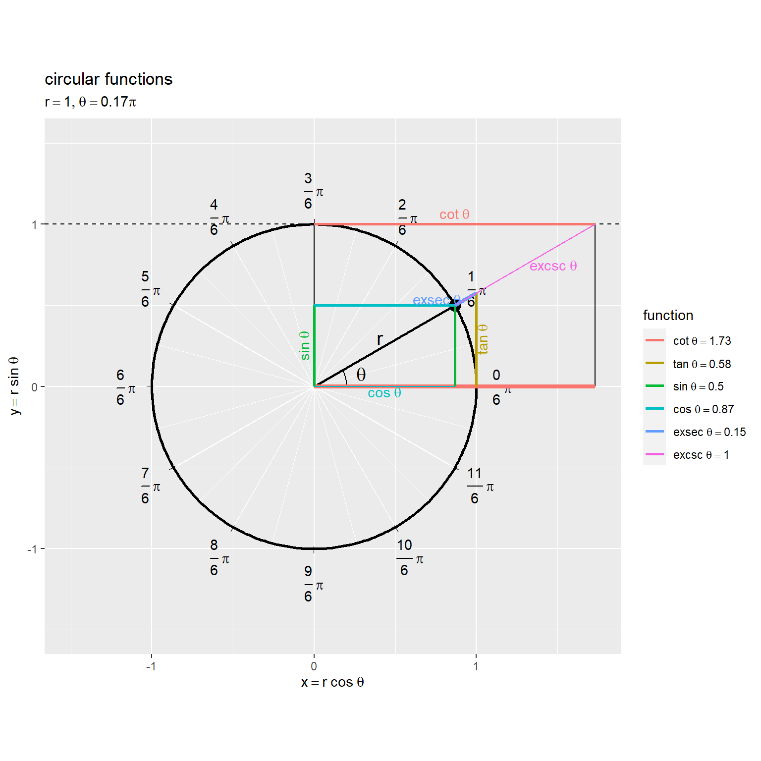
　偏角(始線から動径までの反時計回りの角度)を $\theta$ として、単位円( $r = 1$ の円)の円周上の点の座標は $(x, y) = (\cos \theta, \sin \theta)$ です。
　cot関数の定義式 $\cot \theta = \frac{\cos \theta}{\sin \theta}$ や、この図の相似な直角三角形から、 $\sin \theta : \cos \theta = 1 : \cot \theta$ なのが分かります。 $\theta$ に関する直角三角形について、対辺( $\sin \theta$ に対応する辺)が1になるように拡大したときの隣辺( $\cos \theta$ に対応する辺)と言えます。
　よって、cot関数の値は、「原点と点 $(\cos \theta, \sin \theta)$ を通る半直線」と「 $y = 1$ の直線」の交点のx座標(符号付きの幅)です。

パターン2

　2つ目の方法では、円周上の点から伸びる線分としてcot関数を可視化します。

・作図コード(クリックで展開)

　偏角を示す線分の描画用のデータフレームを作成します。

# 符号の反転フラグを設定
rev_flag <- sin(theta) >= 0

# 半径線の終点の座標を作成
radius_df <- tibble::tibble(
  x = c(1, cos(theta), ifelse(rev_flag, yes = 0, no = NA)), 
  y = c(0, sin(theta), ifelse(rev_flag, yes = 1, no = NA)), 
  w = c("normal", "normal", "thin") # 補助線用
)
radius_df

# A tibble: 3 × 3
      x     y w     
  <dbl> <dbl> <chr> 
1 1       0   normal
2 0.866   0.5 normal
3 0       1   thin

　偏角用の線分の終点(円周上の2点)の座標を格納します。原点 $(0, 0)$ の座標は、作図時に引数に直接指定します。
　また、偏角が $0 \leq \theta \leq \pi$ ( $\sin \theta$ が正の値)のとき、補助線用の線分を追加します。

　関数を示す線分の描画用のデータフレームを作成します。

# 関数の描画順を指定
fnc_level_vec <- c("cot", "tan", "sin", "cos", "exsec", "excsc")

# 関数線分の座標を作成
fnc_seg_df <- tibble::tibble(
  fnc = c(
    "cot", "tan", 
    "sin", "sin", 
    "cos", "cos", 
    "exsec", "excsc"
  ) |> 
    factor(levels = fnc_level_vec), # 関数カテゴリ
  x_from = c(
    cos(theta), cos(theta), 
    0, 0, 
    0, 0, 
    1, 0
  ), 
  y_from = c(
    sin(theta), sin(theta), 
    0, 0, 
    sin(theta), ifelse(rev_flag, yes = 1, no = -1), 
    0, 1
  ), 
  x_to = c(
    0, 1/cos(theta), 
    0, abs(sin(theta))*cos(theta), 
    cos(theta), abs(sin(theta))*cos(theta), 
    1/cos(theta), 0
  ), 
  y_to = c(
    1/sin(theta), 0, 
    sin(theta), abs(sin(theta))*sin(theta), 
    sin(theta), abs(sin(theta))*sin(theta), 
    0, 1/sin(theta)
  ), 
  w = c(
    "normal", "normal", 
    "bold", "normal", 
    "normal", "normal", 
    "normal", "thin"
  ) # 重なり対策用
)
fnc_seg_df

# A tibble: 8 × 6
  fnc   x_from y_from  x_to  y_to w     
  <fct>  <dbl>  <dbl> <dbl> <dbl> <chr> 
1 cot    0.866    0.5 0      2    normal
2 tan    0.866    0.5 1.15   0    normal
3 sin    0        0   0      0.5  bold  
4 sin    0        0   0.433  0.25 normal
5 cos    0        0.5 0.866  0.5  normal
6 cos    0        1   0.433  0.25 normal
7 exsec  1        0   1.15   0    normal
8 excsc  0        1   0      2    thin

　「パターン1」と同様に、線分の座標を格納します。

　関数ラベルの描画用のデータフレームを作成します。

# 関数ラベルの座標を作成
fnc_label_df <- tibble::tibble(
  fnc = c("cot", "tan", "sin", "cos", "exsec", "excsc") |> 
    factor(levels = fnc_level_vec), # 関数カテゴリ
  x = c(
    0.5 * cos(theta), 
    0.5 * (1/cos(theta) + cos(theta)), 
    0, 
    0.5 * cos(theta), 
    0.5 * (1 + 1/cos(theta)), 
    0
  ), 
  y = c(
    0.5 * (1/sin(theta) + sin(theta)), 
    0.5 * sin(theta), 
    0.5 * sin(theta), 
    sin(theta), 
    0, 
    0.5 * (1 + 1/sin(theta))
  ), 
  fnc_label = c("cot~theta", "tan~theta", "sin~theta", "cos~theta", "exsec~theta", "excsc~theta"), 
  a = c( 0,    0,    90,   0,   0,   90), 
  h = c(-0.2, -0.2,  0.5,  0.5, 0.5, 0.5), 
  v = c( 0.5,  0.5, -0.5, -0.5, 1,   1)
)
fnc_label_df

# A tibble: 6 × 7
  fnc       x     y fnc_label       a     h     v
  <fct> <dbl> <dbl> <chr>       <dbl> <dbl> <dbl>
1 cot   0.433  1.25 cot~theta       0  -0.2   0.5
2 tan   1.01   0.25 tan~theta       0  -0.2   0.5
3 sin   0      0.25 sin~theta      90   0.5  -0.5
4 cos   0.433  0.5  cos~theta       0   0.5  -0.5
5 exsec 1.08   0    exsec~theta     0   0.5   1  
6 excsc 0      1.5  excsc~theta    90   0.5   1

　線分の中点の座標とラベル用の文字列などを格納します。

　単位円におけるcot関数のグラフを作成します。

# グラフサイズの下限値・上限値を指定
axis_lower <- 1.5
axis_upper <- 3

# グラフサイズを設定
axis_x_min <- min(-axis_lower, 1/cos(theta)) |> max(-axis_upper)
axis_x_max <- max(axis_lower, 1/cos(theta)) |> min(axis_upper)
axis_y_min <- min(-axis_lower, 1/sin(theta)) |> max(-axis_upper)
axis_y_max <- max(axis_lower, 1/sin(theta)) |> min(axis_upper)

# 単位円における関数線分を作図
ggplot() + 
  geom_segment(data = rad_tick_df, 
               mapping = aes(x = 0, y = 0, xend = x, yend = y, linewidth = grid), 
               color = "white", show.legend = FALSE) + # 角度目盛線
  geom_text(data = rad_tick_df, 
            mapping = aes(x = x, y = y, angle = a, label = tick_mark), 
            size = 2) + # 角度目盛指示線
  geom_text(data = rad_tick_df, 
            mapping = aes(x = label_x, y = label_y, label = rad_label, hjust = h, vjust = v), 
            parse = TRUE) + # 角度目盛ラベル
  geom_path(data = circle_df, 
            mapping = aes(x = x, y = y), 
            linewidth = 1) + # 円周
  geom_segment(data = radius_df, 
               mapping = aes(x = 0, y = 0, xend = x, yend = y, linewidth = w), 
               show.legend = FALSE) + # 半径線
  geom_path(data = angle_mark_df, 
            mapping = aes(x = x, y = y)) + # 角マーク
  geom_text(data = angle_label_df, 
            mapping = aes(x = x, y = y), 
            label = "theta", parse = TRUE, 
            size = 5) + # 角ラベル
  geom_text(mapping = aes(x = 0.5*cos(theta+0.1), y = 0.5*sin(theta+0.1)), 
            label = "r", parse = TRUE, 
            size = 5) + # 半径ラベル:(θ + αで表示位置を調整)
  geom_point(data = point_df, 
             mapping = aes(x = x, y = y), 
             size = 4) + # 円周上の点
  geom_vline(xintercept = 0, linetype = "dashed") + # 補助線
  geom_segment(data = fnc_seg_df, 
               mapping = aes(x = x_from, y = y_from, xend = x_to, yend = y_to, 
                             color = fnc, linewidth = w)) + # 関数線分
  geom_text(data = fnc_label_df, 
            mapping = aes(x = x, y = y, label = fnc_label, color = fnc, 
                          hjust = h, vjust = v, angle = a), 
            parse = TRUE, show.legend = FALSE) + # 関数ラベル
  scale_color_hue(labels = parse(text = fnc_label_vec), name = "function") + # 凡例表示用
  scale_linewidth_manual(breaks = c("bold", "normal", "thin", "major", "minor"), 
                         values = c(1.5, 1, 0.5, 0.5, 0.25)) + # 補助線用, 重なり対策用, 主・補助目盛線用
  guides(color = guide_legend(override.aes = list(linewidth = 1)), 
         linewidth = "none") + 
  theme(legend.text.align = 0) + 
  coord_fixed(ratio = 1, 
              xlim = c(axis_x_min, axis_x_max), 
              ylim = c(axis_y_min, axis_y_max)) + 
  labs(title = "circular functions", 
       subtitle = parse(text = var_label), 
       x = expression(x == r ~ cos~theta), 
       y = expression(y == r ~ sin~theta))

　動径(原点と円周上の点を結ぶ線分)を対辺、y軸線の一部を斜辺としたときのパターン1の図と言えます。文字通り首を捻って見てください。
　円周上の点を $P = (\cos \theta, \sin \theta)$ として、「動径に対する点 $P$ を通る垂線」と「 $x = 0$ の直線」の交点を $Q = (0, \frac{1}{\sin \theta})$ とします。cot関数の値は、点 $P, Q$ を結ぶ線分の符号付きの長さです。

アニメーションの作成

　変数を変化させて、単位円におけるcot関数のアニメーションを作成します。
　作図コードについては「cot_definition.R at anemptyarchive/Mathematics · GitHub」を参照してください。

・パターン1

　 $\theta = n \pi$ ( $n$ は整数)(この図だと $\frac{0}{6} \pi, \frac{6}{6} \pi$ の目盛位置)のとき $\sin \theta = 0$ なので、動径が水平になり直線 $y = 1$ と平行(交点ができない)なため、 $\cot \theta$ を描画(定義)できないのを確認できます。

・パターン2

　こちらの図だと、動径の垂線が垂直になり直線 $x = 0$ と平行なため、 $\cot \theta$ を描画(定義)できないのが分かります。

単位円と曲線の関係

　最後は、単位円と関数曲線のグラフを作成して、変数(ラジアン)と座標の関係を可視化します。
　作図コードについては「cot_definition.R」を参照してください。

変数と座標の関係

　変数に応じて移動する円周上の点と曲線上の点のアニメーションを作成します。

点の座標

　円周上の点とcot関数曲線上の点の関係を可視化します。

　単位円におけるcot関数の値に関して、x軸の値(x軸線上の線分)を正負に応じて回転し、y軸の値(y軸線上の線分)に変換しています。
　 $\sin \theta = 0$ のとき曲線が不連続になり、その前後で符号(線分の向き)が変わるのを確認できます。

　円周上の点とtan関数・cot関数曲線上の点の関係を可視化します。

　左下図によってx座標(横方向の線分)からy座標(縦方向の線分)に変換(回転)し、tan関数とcot関数の曲線を並べて比較します。
　tan関数の値は動径の延長線と直線 $x = 1$ の交点のy座標(符号付きの高さ)です。

点の推移

　円周上を周回した際のcot関数の推移を可視化します。

　単位円を半周する $\pi$ の間隔で、曲線の形状が一致するのを確認できます。

　円周上を周回した際のtan関数・cot関数の推移を可視化します。

　この記事では、cot関数の定義を確認しました。次の記事からは、各種パラメータによる波形への影響を確認していきます。または、sec関数の定義を確認します。

参考書籍

『三角関数(改定第3版)』(Newton別冊)ニュートンプレス,2022年.

おわりに

　secとcscでそれぞれ1か所悩んでいる部分がありまして、先にcotを完成させました。
　気温が上がってきてやる気が下がってきており、前回から半月空いてしまいました。なんだかもう色々面倒臭いです。梅雨が過ぎたら冬が来てほしい。

2024.03.21：加筆修正しますた。

　どーでもいー細かい話ですが、今回の修正前までは(双曲線関数のシリーズでも)sin→cos→tan→sec→csc→cotの順で構成していました。理解が進んでtanとcotはセットだよなと順番を入れ替えました。
　さらにだから何って話ですが、修正前の記事では11万字を超えていました。流石に読み手にも書き手にも大変だよね。修正後は3万字になりました。ほとんどは重複するコードなのでこの記事の解説だけで分かると思うので、アニメーションを作りたい方はGitHubを覗いてみてください。

【次の内容】

からっぽのしょこ

読んだら書く！書いたら読む！同じ事は二度調べ(たく)ない

【R】cot関数の定義の可視化

はじめに

cot関数の定義の可視化

定義式の確認

曲線の形状

曲線の作成

単位円の作成

単位円と関数の関係

グラフの作成

パターン1

パターン2

アニメーションの作成

単位円と曲線の関係

変数と座標の関係

点の座標

点の推移

参考書籍

おわりに