はじめに

　gganimateパッケージについて理解したいシリーズです。
　この記事では、Quintic関数によるイージング処理を解説します。

【他の内容】

【目次】

はじめに
Quintic
おわりに

Quintic

　5次イージング関数(Quintic Easing Function)とイージング処理についてアニメーションで確認します。

　利用するパッケージを読み込みます。

# 利用パッケージ
library(gganimate)
library(tidyverse)

　基本的に、パッケージ名::関数名()の記法で書きます。ただし作図コードに関してはごちゃごちゃしてしまうので、ggplot2パッケージの関数は関数名のみで、gganimateパッケージの関数はパッケージ名を明示して書きます。

5次関数の確認

　5次イージング関数(Quintic関数)は、5次関数(Quintic Function)を利用します。

$f(x) = x^5$

　この関数をグラフで確認します。

・作図コード(クリックで展開)

　x軸の値と関数の出力(y軸の値)をデータフレームに格納します。

# x軸の値を作成
x_vec <- seq(from = -1.1, to = 1.1, by = 0.01)

# 5次関数
tmp_df <- tibble::tibble(
  x = x_vec, 
  y = x^5
)

　このデータフレームはここでしか使いません。

　イージング関数として利用する範囲を示すのに利用するデータフレームを作成します。

# イージング関数として利用する領域
area_df <- tibble::tibble(
  x_from = c(0, 0, 1, 1), 
  y_from = c(0, 1, 1, 0), 
  x_to = c(0, 1, 1, 0), 
  y_to = c(1, 1, 0, 0)
)

　点 $(x, y)$ として、4つの点 $(0, 0)$ ・ $(0, 1)$ ・ $(1, 1)$ ・ $(1, 0)$ に対応します。

　5次関数のグラフを作成します。

# 5次関数を作図
ggplot() + 
  geom_line(data = tmp_df, mapping = aes(x = x, y = y), 
            color = "hotpink", size = 1) + # 元の関数
  geom_segment(data = area_df, mapping = aes(x = x_from, xend = x_to, y = y_from, yend = y_to), 
               color = "red", size = 1) + # 対象の領域
  coord_fixed(ratio = 1) + # アスペクト比
  labs(title = expression(f(x) == x^5), 
       y = expression(f(x)))

　geom_segment()で領域を描きます。x, y引数に指定した点とxend, yend引数に指定した点を直線で繋ぎます。

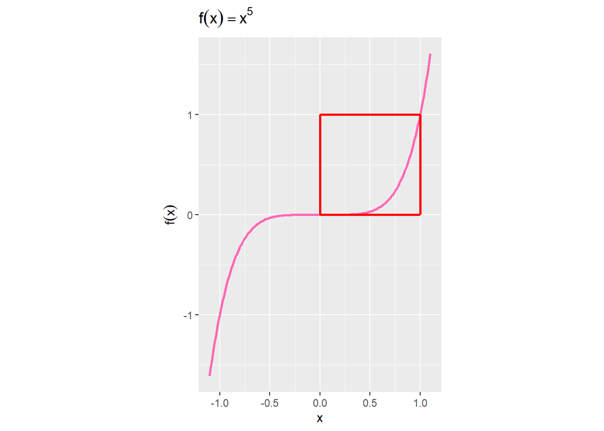
f:id:anemptyarchive:20220409150112p:plain — 5次関数のグラフ

　イージング関数では、赤色の線で囲まれた縦横0から1の領域に注目します。

In

　まずは、Quintic-inイージング関数を確認します。Inタイプは、始めの変化が小さく、時間が進むにつれて変化が大きくなります。

　Quint-in関数は、次の式で定義されます。

$f_{in}(t) = t^5 \quad (0 \leq t \leq 1)$

　 $0 \leq t \leq 1$ のとき $0 \leq f(t) \leq 1$ になるのが先ほどのグラフからも分かります。

　この関数(y軸の値)を計算して、時間(x軸)の値と共にデータフレームに格納します。

# 時間変化の値を作成:(0 <= t <= 1)
t_vec <- seq(from = 0, to = 1, by = 0.01)

# Quintic-in
quint_in_df <- tibble::tibble(
  t = t_vec, 
  y = t^5, 
  easing_fnc = "quint-in"
)
head(quint_in_df)

## # A tibble: 6 x 3
##       t            y easing_fnc
##   <dbl>        <dbl> <chr>     
## 1  0    0            quint-in  
## 2  0.01 0.0000000001 quint-in  
## 3  0.02 0.0000000032 quint-in  
## 4  0.03 0.0000000243 quint-in  
## 5  0.04 0.000000102  quint-in  
## 6  0.05 0.000000313  quint-in

　他の関数と比較する際に利用するため、easing_fnc列として関数名を持たせておきます。

　作図用のデータフレームを作成します。

# イージング関数を指定
point_df <- quint_in_df

# イージング曲線用のデータフレームを作成
line_df <- point_df %>% 
  dplyr::rename(x = t) # フレーム用の列をx軸用の列に変更

　作図コードを再利用しやすいように、グラフを描画する関数のデータフレームをpoint_dfとして複製します。この後作成する他の関数のデータフレームを指定すると、その関数のグラフを同じコードで描画できます(タイトルは書き換えます)。
　ここでは、時間(t列の値)の変化に応じてフレームを切り替えるアニメーションを作成します。アニメーション(フレーム切替)の影響を受けずにイージング曲線(折れ線グラフ)を描画するために、フレーム列(x軸の値の列)の名前を変更しておきます。

　Quint-in関数のアニメーションを作成します。

# イージング関数を作図
anim <- ggplot(point_df, aes(x = t, y = y)) + 
  geom_line(data = line_df, mapping = aes(x = x, y = y), 
            color = "hotpink", size = 1) + # イージング曲線
  geom_vline(mapping = aes(xintercept = t), 
             color = "orange", size = 1, linetype = "dashed") + # 経過時間の線
  geom_hline(mapping = aes(yintercept = y), 
             color = "red", size = 1, linetype = "dashed") + # 変化量の線
  geom_point(mapping = aes(y = 0), color = "orange", size = 5) + # 経過時間の点
  geom_point(mapping = aes(x = 1), color = "red", size = 5) + # 変化量の点
  geom_point(color = "hotpink", size = 5) + # イージング曲線上の点
  gganimate::transition_reveal(along = t) + # フレーム
  coord_fixed(ratio = 1) + # アスペクト比
  labs(title = "Quintic-in Easing Function", 
       subtitle = "t = {round(frame_along, 2)}", 
       color = "easing function", 
       x = "time", y = expression(f(t)))

# gif画像を作成
gganimate::animate(plot = anim, nframes = 50, fps = 20)

f:id:anemptyarchive:20220409150124g:plain — Quintic-in関数のグラフ

　x軸上を通過するオレンジ色の点は、経過時間を表します。この点(時間経過)は、常に一定に変化します。
　ピンク色の線は、イージング関数のグラフで、経過時間と移動量(アニメーションの変化)の関係を表します。イージング曲線上を通過するピンク色の点は、その時間における関数の値です。
　y軸に対して並行に移動する赤色の点は、イージング関数に従って変化する点で、イージング処理されたアニメーションの変化を表します。

　Quint-in関数によるイージング処理は、時間が経つほど変化が大きくなるのが分かります。

Out

　次は、Quintic-outイージング関数を確認します。Outタイプは、始めの変化が大きく、時間が進むにつれて変化が小さくなります。

　Quint-out関数は、Inの関数を用いて次の式で定義されます。

$f_{out}(t) = 1 - f_{in}(1 - t) \quad (0 \leq t \leq 1)$

　時間 $t$ は0から1に変化するので、 $1 - t$ は0から1に変化します。この操作により、y軸に対してグラフが反転します。
　さらに、 $f_{in}(1 - t)$ は1から0に変化するので、 $1 - f_{in}(1 - t)$ は0から1に変化します。これにより、x軸に対してもグラフが反転した関数が得られます。

　この式を整理します。Inの式の $t$ を $t'$ で表し $1 - t$ に置き換えると

$\begin{aligned} f_{out}(t) &= 1 - (t')^5 \\ &= 1 - (1 - t)^5 \end{aligned}$

で計算できることが分かります。
　また、 $- x^5 = (- x)^5$ なので、括弧に $- 1$ を入れて

$f_{out}(t) = 1 + (t + 1)^5$

でも計算できます。

　時間(x軸)の値とイージング関数(y軸)の値をデータフレームに格納します。

# Quintic-out
quint_out_df <- tibble::tibble(
  t = t_vec, 
  y = 1 - (1 - t)^5, 
  easing_fnc = "quint-out"
)
head(quint_out_df)

## # A tibble: 6 x 3
##       t      y easing_fnc
##   <dbl>  <dbl> <chr>     
## 1  0    0      quint-out 
## 2  0.01 0.0490 quint-out 
## 3  0.02 0.0961 quint-out 
## 4  0.03 0.141  quint-out 
## 5  0.04 0.185  quint-out 
## 6  0.05 0.226  quint-out

　Quint-out関数のアニメーションを作成します。

f:id:anemptyarchive:20220409150156g:plain — Quintic-out関数のグラフ

　Quint-out関数によるイージング処理は、時間が経つほど変化が小さくなるのが分かります。

InOut

　続いて、Quintic-in-outイージング関数を確認します。InOutタイプは、始めと終わりの変化が小さく、中盤の変化が大きくなります。

　Quint-in-out関数は、Inの関数とOutの関数を用いて次の式で定義されます。

$\begin{aligned} f_{inout}(t) = \begin{cases} \frac{1}{2} f_{in}(2 t) &\quad (0 \leq t < 0.5) \\ \frac{1}{2} (f_{out}(2 t - 1) + 1) &\quad (0.5 \leq t \leq 1) \end{cases} \end{aligned}$

　前半( $t$ が0から0.5の間)の変化ではInの関数で計算します。 $t$ を2倍にすることで0から1の範囲で関数の計算を行い、計算結果を2分の1にすることで出力を0から0.5の範囲に抑えます。
　後半( $t$ が0.5から1の間)の変化ではOutの関数で計算します。こちらも $2 t - 1$ にすることで0から1の範囲で関数の計算を行い、前半部分に対応する(2分の1になるので0.5の2倍の)1を足して、2分の1にすることで出力を0.5から1の範囲にします。

　それぞれ式を整理します。上の式(前半の式)は、Inの式の $t$ を $t'$ で表し $2 t$ に置き換えて

$\begin{aligned} \frac{1}{2} f_{in}(2 t) &= \frac{1}{2} (t')^5 \\ &= \frac{1}{2} (2 t)^5 \\ &= \frac{1}{2} 2^5 t^5 \\ &= 16 t^5 \end{aligned}$

となります。

　下の式(後半の式)は、Outの関数の $t$ を $t'$ で表し $2 t - 1$ に置き換えて

$\begin{aligned} \frac{1}{2} (f_{out}(2 t - 1) + 1) &= \frac{1}{2} \Bigl\{ 1 - (1 - t')^5 + 1 \Bigr\} \\ &= \frac{1}{2} \Bigl[ 2 - \{1 - (2 t - 1)\}^5 \Bigr] \\ &= \frac{1}{2} \Bigl\{ 2 - (2 - 2 t)^5 \Bigr\} \\ &= 1 - \frac{(2 - 2 t)^5}{2} \end{aligned}$

となります。

　よって、2つの式をまとめると

$\begin{aligned} f_{inout}(t) = \begin{cases} 16 t^5 &\quad (0 \leq t < 0.5) \\ 1 - \frac{(2 - 2 t)^5}{2} &\quad (0.5 \leq t \leq 1) \end{cases} \end{aligned}$

で計算できます。

　時間(x軸)の値とイージング関数(y軸)の値をデータフレームに格納します。

# Quintic-inout
quint_inout_df <- tibble::tibble(
  t = t_vec, 
  y = dplyr::if_else(
    condition = t < 0.5, 
    true = 16 * t^5, 
    false = 1 - (2 - 2 * t)^5 * 0.5
  ), 
  easing_fnc = "quint-in-out"
)
head(quint_inout_df)

## # A tibble: 6 x 3
##       t            y easing_fnc  
##   <dbl>        <dbl> <chr>       
## 1  0    0            quint-in-out
## 2  0.01 0.0000000016 quint-in-out
## 3  0.02 0.0000000512 quint-in-out
## 4  0.03 0.000000389  quint-in-out
## 5  0.04 0.00000164   quint-in-out
## 6  0.05 0.000005     quint-in-out

　dplyrパッケージのif_else()を使って、場合分けして計算します。

　Quint-in-out関数のアニメーションを作成します。

f:id:anemptyarchive:20220409150219g:plain — Quintic-in-out関数のグラフ

　Quint-in-out関数によるイージング処理は、中ごろで大きく変化するのが分かります。

イージング処理の比較

　最後に、Linear関数と3つのQuintic関数を比較します。

　これまでに確認したグラフを重ねて描画するため、データフレームを結合します。

# linear
linear_df <- tibble::tibble(
  t = t_vec, 
  y = t, 
  easing_fnc = "linear"
)

# 比較対象を結合
easing_df <- rbind(
  linear_df, 
  quint_in_df, 
  quint_out_df, 
  quint_inout_df
) %>% 
  dplyr::mutate(
    easing_fnc = factor(easing_fnc, level = c("linear", "quint-in", "quint-out", "quint-in-out"))
  ) # 因子型に変換

# イージング曲線用のデータフレームを作成
line_df <- easing_df %>% 
  dplyr::rename(x = t) # フレーム用の列をx軸用の列に変更

# 確認
head(easing_df)

## # A tibble: 6 x 3
##       t     y easing_fnc
##   <dbl> <dbl> <fct>     
## 1  0     0    linear    
## 2  0.01  0.01 linear    
## 3  0.02  0.02 linear    
## 4  0.03  0.03 linear    
## 5  0.04  0.04 linear    
## 6  0.05  0.05 linear

　比較する関数のデータフレームを結合します。
　グラフを色分けするために、関数名の列を因子型に変換しておきます。factor()のレベル引数levelに関数名の順番を指定すると、凡例の並びや色付けを指定できます。

　イージング関数のアニメーションを作成します。

# イージング関数を作図
anim <- ggplot(easing_df, aes(x = t, y = y, color = easing_fnc)) + 
  geom_vline(mapping = aes(xintercept = t), 
             color = "pink", size = 1, linetype = "dashed") + # 経過時間の線
  geom_hline(mapping = aes(yintercept = y, color = easing_fnc), linetype = "dashed") + 
  geom_line(data = line_df, mapping = aes(x = x, y = y, color = easing_fnc), size = 1) + # イージング曲線
  geom_point(mapping = aes(x = 1), size = 5) + 
  geom_point(mapping = aes(y = 0), color = "pink", size = 5) + 
  geom_point(size = 5) + # イージング曲線上の点
  gganimate::transition_reveal(along = t) + # フレーム
  scale_color_manual(values = c("red", "limegreen", "orange", "mediumblue")) + # 点と線の色:(不必要)
  coord_fixed(ratio = 1) + # アスペクト比
  labs(title = "Quintic Easing Functions", 
       subtitle = "t = {round(frame_along, 2)}", 
       color = "easing function", 
       x = "time", y = expression(f(t))) # ラベル

# gif画像を作成
gganimate::animate(plot = anim, nframes = 50, fps = 20)

f:id:anemptyarchive:20220409150246g:plain — Quintic関数のグラフ

　InのグラフとOutのグラフが点 $(0.5, 0.5)$ で点対称になっているのが分かります。また、InOutのグラフがInとOutを繋げたグラフになっており、点 $(0.5, 0.5)$ でLinear関数と等しくなるのが分かります。

　続いて、垂直に移動する点で表現していたイージング処理された変化を、棒グラフで表現します。

# イージング関数の数を取得
fnc_size <- length(unique(easing_df[["easing_fnc"]]))

# イージングバー用のデータフレームを作成
bar_df <- easing_df %>% 
  dplyr::mutate(x = (rep(1:fnc_size, each = length(t_vec)) * 2 - 1) / (fnc_size * 2)) # x軸の値を等間隔に設定
head(bar_df)

## # A tibble: 6 x 4
##       t     y easing_fnc     x
##   <dbl> <dbl> <fct>      <dbl>
## 1  0     0    linear     0.125
## 2  0.01  0.01 linear     0.125
## 3  0.02  0.02 linear     0.125
## 4  0.03  0.03 linear     0.125
## 5  0.04  0.04 linear     0.125
## 6  0.05  0.05 linear     0.125

　バーを0から1の範囲で等間隔に配置するために、x軸の値を等間隔に設定します。

　棒グラフのアニメーションを作成します。

# イージング処理を作図
anim <- ggplot() + 
  geom_tile(data = bar_df, mapping = aes(x = x, y = y/2, height = y, fill = easing_fnc), 
           alpha = 0.7, width = 0.9/fnc_size) + # イージングバー
  geom_hline(data = easing_df, mapping = aes(yintercept = y, color = easing_fnc), 
             linetype = "dashed") + # 変化量の線
  geom_line(data = line_df, mapping = aes(x = x, y = y, color = easing_fnc)) + # イージング曲線
  geom_point(data = easing_df, mapping = aes(x = t, y = y, color = easing_fnc), 
             alpha = 0.5, size = 5) + # イージング曲線上の点
  gganimate::transition_reveal(along = t) + # フレーム
  scale_color_manual(values = c("red", "limegreen", "orange", "mediumblue")) + # 点と線の色:(不必要)
  scale_fill_manual(values = c("red", "limegreen", "orange", "mediumblue")) + # バーの色:(不必要)
  coord_fixed(ratio = 1) + # アスペクト比
  labs(title = "Quintic Easing Functions", 
       subtitle = "t = {round(frame_along, 2)}", 
       fill = "easing function", color = "easing function", 
       x = "time", y = expression(f(x))) # ラベル

# gif画像を作成
gganimate::animate(plot = anim, nframes = 50, fps = 20)

f:id:anemptyarchive:20220409150255g:plain — Quintic関数によるイージング処理

　イージング曲線上の点と対応するバーの高さが一致しているのが分かります。

　点の軌跡でイージング処理を可視化します。

　作図用にデータフレームを加工します。(それとは別に、時間の値を粗く(by = 0.1に)してデータを作り直しました。)

# イージング関数の数を取得
fnc_size <- length(unique(easing_df[["easing_fnc"]]))

# 移動点用のデータフレームを作成
point_df <- easing_df %>% 
  dplyr::mutate(
    x = rep(1:fnc_size, each = length(t_vec)), 
    frame = t
  ) %>% # プロット位置とフレーム列を追加
  dplyr::select(t, x, y, easing_fnc, frame) # 列を並べ替え

# 最初のフレームで描画するデータを確認
point_df %>% 
  dplyr::filter(frame == 0)

## # A tibble: 4 x 5
##       t     x     y easing_fnc   frame
##   <dbl> <int> <dbl> <fct>        <dbl>
## 1     0     1     0 linear           0
## 2     0     2     0 quint-in         0
## 3     0     3     0 quint-out        0
## 4     0     4     0 quint-in-out     0

　点のプロット位置として、関数ごとにx軸の値を割り当てます。また、フレーム列として時間列の値を複製します。

　過去の点の位置を表示するために、データ(行)を複製したデータフレームを作成します。

# 点の軌跡用のデータフレームを作成
trace_point_df <- easing_df %>% 
  tibble::add_column(
    x = rep(1:fnc_size, each = length(t_vec)), 
    n = rep((length(t_vec)-1):0, times = fnc_size)
  ) %>% # 複製する数を追加
  tidyr::uncount(n) %>% # 過去フレーム用に複製
  dplyr::group_by(t, easing_fnc) %>% # 時間と関数でグループ化
  dplyr::mutate(
    idx = length(t_vec) + 1 - dplyr::row_number(), 
    frame = t_vec[idx]
  ) %>% # フレーム列を追加
  dplyr::ungroup() %>% # グループ化を解除
  dplyr::arrange(frame, x) %>% # 昇順に並び替え
  dplyr::select(t, x, y, easing_fnc, frame) # 利用する列を選択

# 第3フレームまでに描画するデータ
trace_point_df %>% 
  dplyr::filter(frame <= 0.2)

## # A tibble: 12 x 5
##        t     x       y easing_fnc   frame
##    <dbl> <int>   <dbl> <fct>        <dbl>
##  1   0       1 0       linear         0.1
##  2   0       2 0       quint-in       0.1
##  3   0       3 0       quint-out      0.1
##  4   0       4 0       quint-in-out   0.1
##  5   0       1 0       linear         0.2
##  6   0.1     1 0.1     linear         0.2
##  7   0       2 0       quint-in       0.2
##  8   0.1     2 0.00001 quint-in       0.2
##  9   0       3 0       quint-out      0.2
## 10   0.1     3 0.410   quint-out      0.2
## 11   0       4 0       quint-in-out   0.2
## 12   0.1     4 0.00016 quint-in-out   0.2

　この例だと、最初のフレーム(frame列が0)ではデータがなく、2番目のフレーム(frame列が0.1)では前の時間(t列が0)のデータ、3番目のフレーム(frame列が0.2)ではそれまでの時間(t列が0.2未満)のデータとなるようにします。

　横方向に点が移動するアニメーションを作成します。

# イージングされた点移動を作図
anim <- ggplot(point_df, aes(x = x, y = y, color = easing_fnc)) + 
  geom_hline(mapping = aes(yintercept = t), 
             color = "pink", size = 1, linetype = "dashed") + # 経過時間の線
  geom_point(size = 5, show.legend = FALSE) + # イージング移動点
  geom_point(data = trace_point_df, mapping = aes(x = x, y = y, color = easing_fnc), 
             size = 5, alpha = 0.2, show.legend = FALSE) + # 点の軌跡
  gganimate::transition_manual(frame = frame) + # フレーム
  scale_x_reverse(breaks = unique(point_df[["x"]]), labels = unique(point_df[["easing_fnc"]]), minor_breaks = FALSE) + # x軸目盛の反転
  scale_color_manual(values = c("red", "limegreen", "orange", "mediumblue")) + # 点と線の色:(不必要)
  scale_fill_manual(values = c("red", "limegreen", "orange", "mediumblue")) + # 点と線の色:(不必要)
  coord_flip() + # 軸の入れ替え
  labs(title = "Quintic Easing Functions", 
       subtitle = "t = {current_frame}", 
       x = "Easing Function", y = expression(f(t)))

# gif画像を作成
gganimate::animate(plot = anim, nframes = length(t_vec)+10, fps = 10, end_pause = 10)

f:id:anemptyarchive:20220409150311g:plain — Quintic関数によるイージング処理

　coord_flip()でx軸とy軸を入れ変えているので、横方向がy軸になります。

　変化が遅い地点(時間)ほど点の跡が多く残ります。点の跡の偏りがイージング曲線に対応します。

　以上で、5次イージング関数を確認しました。次は、指数イージング関数を確認します。

おわりに

　ここまではほぼ同じ関数だったので飽きつつありましたが、次からはまた別の関数なので面白いといいですね。

【次の内容】

からっぽのしょこ

読んだら書く！書いたら読む！同じ事は二度調べ(たく)ない

Quintic関数によるイージング【gganimate】