はじめに
R言語で三角関数の定義や公式を可視化しようシリーズのスピンオフです。
この記事では、双曲線関数のグラフを作成します。
【前の内容】
【他の記事一覧】
【この記事の内容】
双曲線関数の可視化
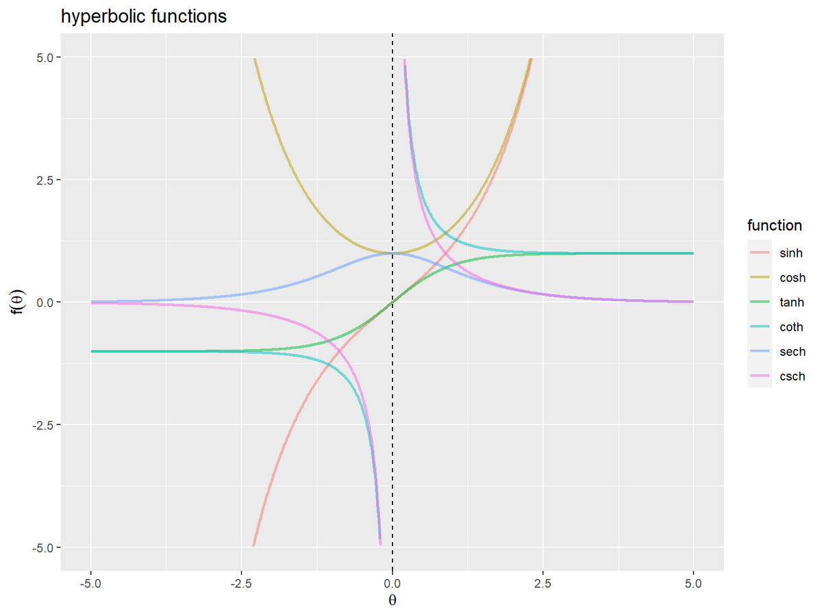
6つ双曲線関数(sinh関数・cosh関数・tanh関数・csc関数・sech関数・coth関数)をグラフで確認します。
利用するパッケージを読み込みます。
# 利用パッケージ
library(tidyverse)
library(patchwork)
library(gganimate)
library(magick)
この記事では、基本的にパッケージ名::関数名()の記法を使うので、パッケージを読み込む必要はありません。ただし、作図コードがごちゃごちゃしないようにパッケージ名を省略しているためggplot2を読み込む必要があります。
また、ネイティブパイプ演算子|>を使っています。magrittrパッケージのパイプ演算子%>%に置き換えても処理できますが、その場合はmagrittrも読み込む必要があります。
定義式の確認
まずは、双曲線関数の定義式を確認します。
双曲線関数は、それぞれsinh関数またはcosh関数を用いて、次の式で定義されます。
$e^x$はネイピア数$e$を底とする自然指数関数です。各関数についてはそれぞれの記事をこちらのページ「Rによる三角関数(円関数)入門:記事一覧 - からっぽのしょこ」から参照してください。
双曲線関数曲線の作図
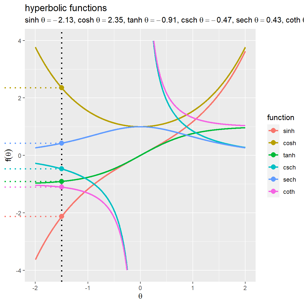
次に、6つの双曲線関数のグラフを作成します。
作図用の変数の値を作成します。
# 作図用の変数の値を指定
theta_vec <- seq(from = -5, to = 5, by = 0.01)
head(theta_vec)
## [1] -5.00 -4.99 -4.98 -4.97 -4.96 -4.95
作図に利用する変数$\theta$の範囲と間隔を指定してtheta_vecとします。
・作図コード(クリックで展開)
双曲線関数の曲線を描画するためのデータフレームを作成します。
# 閾値を指定
threshold <- 5

# 関数ラベルのレベルを指定
fnc_level_vec <- c("sinh", "cosh", "tanh", "coth", "sech", "csch")

# 双曲線関数曲線の描画用
function_df <- tibble::tibble(
  t = rep(theta_vec, times = 6),
  f_t = c(
    sinh(theta_vec), cosh(theta_vec), tanh(theta_vec),
    1/sinh(theta_vec), 1/cosh(theta_vec), 1/tanh(theta_vec)
  ),
  fnc = c("sinh", "cosh", "tanh", "csch", "sech", "coth") |>
    rep(each = length(theta_vec)) |>
      factor(levels = fnc_level_vec), # 色分け用
) |>
  dplyr::mutate(
    f_t = dplyr::if_else(
      (f_t >= -threshold & f_t <= threshold), true = f_t, false = as.numeric(NA)
    )
  ) # 描画範囲外を欠損値に置換
function_df
## # A tibble: 6,006 × 3
##        t   f_t fnc
##    <dbl> <dbl> <fct>
##  1 -5       NA sinh
##  2 -4.99    NA sinh
##  3 -4.98    NA sinh
##  4 -4.97    NA sinh
##  5 -4.96    NA sinh
##  6 -4.95    NA sinh
##  7 -4.94    NA sinh
##  8 -4.93    NA sinh
##  9 -4.92    NA sinh
## 10 -4.91    NA sinh
## # … with 5,996 more rows
$\theta$の値と各関数の値をデータフレームに格納します。sinh関数はsinh()、cosh関数はcosh()、tanh関数はtanh()で計算できます。
関数によっては、0付近で$-\infty$または$\infty$に近付くので、閾値thresholdを指定しておき、-threshold未満またはthresholdより大きい場合は(数値型の)欠損値NAに置き換えます。
双曲線関数のグラフを作成します。
# 双曲線関数数曲線を作図
ggplot() +
  geom_line(data = function_df, mapping = aes(x = t, y = f_t, color = fnc),
            size = 1, alpha = 0.5) + # 双曲線関数曲線
  geom_vline(xintercept = 0, linetype = "dashed") + # 漸近線
  labs(title = "hyperbolic functions",
       color = "function",
       x = expression(theta), y = expression(f(theta)))
x軸を$\theta$、y軸を各関数の値として、geom_line()で折れ線グラフを描画します。
また、$x = 0$の漸近線をgeom_vline()で描画します。
双曲線の作図
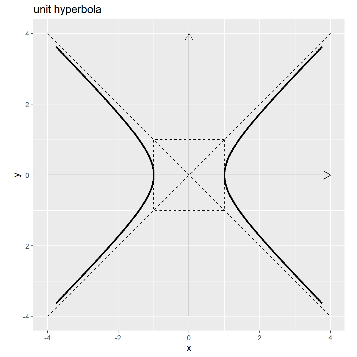
続いて、双曲線関数の可視化に利用する単位双曲線(unit hyperbola)のグラフを作成します。双曲線については「【R】双曲線の作図 - からっぽのしょこ」を参照してください。
・作図コード(クリックで展開)
作図に利用するデータフレームを作成します。
# 作図用の変数の値を指定
theta_vec <- seq(from = -2, to = 2, by = 0.002)

# 双曲線の描画用
hyperbola_df <- tibble::tibble(
  t = c(theta_vec, theta_vec),
  sinh_t = c(sinh(theta_vec), sinh(theta_vec)),
  cosh_t = c(cosh(theta_vec), -cosh(theta_vec)),
  sign = rep(c("plus", "minus"), each = length(theta_vec))# 符号
)

# 軸の最大値を設定
axis_max <- hyperbola_df[["cosh_t"]] |>
  max() |>
  ceiling()

# 漸近線の描画用
asymptote_df <- tibble::tibble(
  x = seq(from = -axis_max, to = axis_max, length.out = 100) |>
    rep(times = 2),
  y = rep(c(1, -1), each = 100) * x,
  slope = rep(c("plus", "minus"), each = 100) # 符号
)

# 正方形グリッドの描画用
square_df <- tibble::tibble(
  x = c(1, 1, -1, -1, 1),
  y = c(1, -1, -1, 1, 1)
)

# 軸線の描画用
axis_df <- tibble::tibble(
  x_from = c(-axis_max, 0),
  y_from = c(0, -axis_max),
  x_to = c(axis_max, 0),
  y_to = c(0, axis_max),
  axis = c("x", "y")
)
双曲線と補助線のグラフを作成します。
# 単位双曲線を作図
ggplot() +
  geom_segment(data = axis_df,
               mapping = aes(x = x_from, y = y_from, xend = x_to, yend = y_to, group = "axis"),
               arrow = arrow(length = unit(10, units = "pt"))) + # 軸線
  geom_path(data = square_df,
            mapping = aes(x = x, y = y), linetype = "dashed") + # 正方形グリッド
  geom_line(data = asymptote_df,
            mapping = aes(x = x, y = y, group = slope), linetype = "dashed") + # 漸近線
  geom_path(data = hyperbola_df,
            mapping = aes(x = cosh_t, y = sinh_t, group = sign),
            size = 1) + # 双曲線
  theme(legend.text.align = 0.5) + # 凡例の体裁:(凡例表示用)
  coord_fixed(ratio = 1,
              xlim = c(-axis_max, axis_max), ylim = c(-axis_max, axis_max)) + # 表示範囲
  labs(title = "unit hyperbola",
       x = "x", y = "y")
このグラフ上に双曲線関数を描画します。
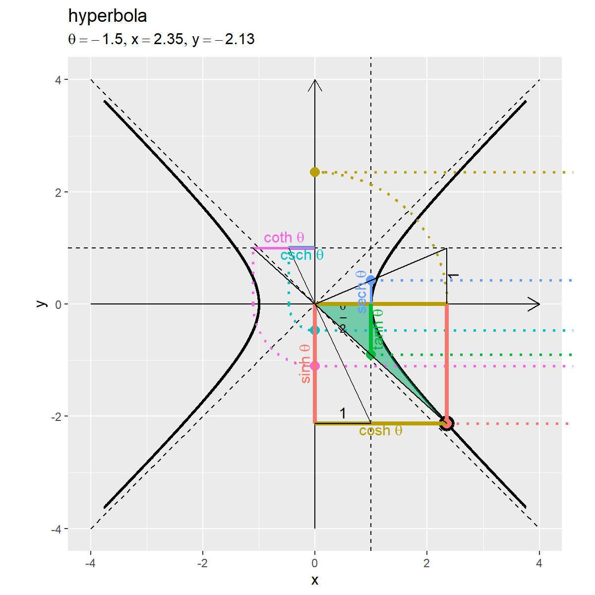
双曲線上の双曲線関数の可視化
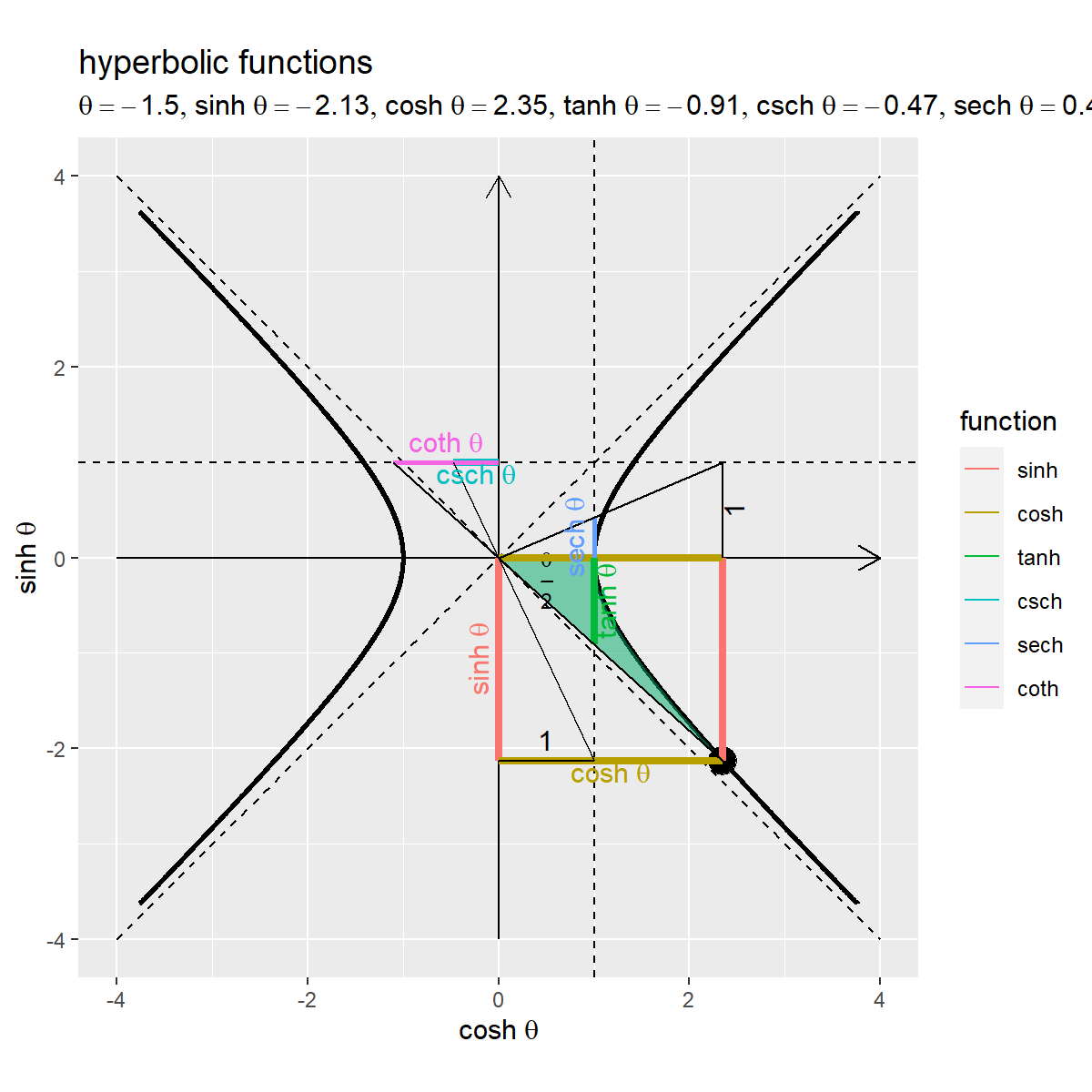
次は、単位双曲線上における双曲線関数(sinh・cosh・tanh・csch・sech・toch)のグラフを作成します。
グラフの作成
変数を固定した双曲線関数をグラフで確認します。
変数の値を設定します。
# 変数の値を指定
theta <- -1.5
変数$\theta$の値を指定します。
・作図コード(クリックで展開)
双曲線上の点を描画するためのデータフレームを作成します。
# 双曲線上の点の描画用
hyperbola_point_df <- tibble::tibble(
  t = theta,
  x = cosh(theta),
  y = sinh(theta),
)
hyperbola_point_df
## # A tibble: 1 × 3
##       t     x     y
##   <dbl> <dbl> <dbl>
## 1  -1.5  2.35 -2.13
単位双曲線上の点のx軸の値$\cosh \theta$とy軸の値$\sinh \theta$を格納します。
変数の値(の半分)を面積(塗りつぶし領域)として描画するためのデータフレームを作成します。
# 変数(面積)の描画用
variable_area_df <- tibble::tibble(
  x = seq(from = 0, to = cosh(theta), length.out = 50),
  sign = dplyr::if_else(theta >= 0, true = 1, false = -1), # 符号
  curve = sign * sqrt(x^2 - 1), # x軸と双曲線上の線分
  straight = sinh(theta)/cosh(theta) * x # 原点と曲線上の点の線分
) |>
  dplyr::mutate(
    curve = dplyr::if_else(is.na(curve), true = 0, false = curve)
  ) # 双曲線の範囲外を0に置換
variable_area_df
## # A tibble: 50 × 4
##         x  sign curve straight
##     <dbl> <dbl> <dbl>    <dbl>
##  1 0         -1     0   0
##  2 0.0480    -1     0  -0.0435
##  3 0.0960    -1     0  -0.0869
##  4 0.144     -1     0  -0.130
##  5 0.192     -1     0  -0.174
##  6 0.240     -1     0  -0.217
##  7 0.288     -1     0  -0.261
##  8 0.336     -1     0  -0.304
##  9 0.384     -1     0  -0.348
## 10 0.432     -1     0  -0.391
## # … with 40 more rows
「原点と双曲線上の点を結ぶ線分」と「$0 \leq x < 1$の範囲のx軸線($y = 0$の直線)と$1 \leq x \leq \cosh \theta$の範囲の双曲線」の範囲を塗りつぶします。ただし、双曲線について、$\theta > 0$のときは$y > 0$の範囲を塗りつぶすため$y = \sqrt{x^2 - 1}$、$\theta < 0$のときは$y < 0$の範囲を塗りつぶすため$y = - \sqrt{x^2 - 1}$を使います。
x軸の値として$0$から$\cosh \theta$の範囲の値を作成してx列とします。
thetaの正負によって符号を変更してsign列としておき、双曲線を計算してcurve列とします。ただし、$0$から$1$の範囲がNaNになるので0に置き換えます。
原点と点$(\cosh \theta, \sinh \theta)$を結ぶ直線の傾きは$a = \frac{\sinh \theta}{\cosh \theta}$です。$y = a x$を計算してstraight列とします。
双曲線関数を直線として描画するためのデータフレームを作成します。
# 関数ラベルのレベルを指定
fnc_level_vec <- c("sinh", "cosh", "tanh", "csch", "sech", "coth")

# 双曲線関数直線の描画用
function_line_df <- tibble::tibble(
  x_from = c(
    0, cosh(theta), 0, 0, 1,
    0, 1, 0
  ),
  y_from = c(
    0, 0, 0, sinh(theta), 0,
    1, 0, 1
  ),
  x_to = c(
    0, cosh(theta), cosh(theta), cosh(theta), 1,
    1/sinh(theta), 1, 1/tanh(theta)
  ),
  y_to = c(
    sinh(theta), sinh(theta), 0, sinh(theta), tanh(theta),
    1, 1/cosh(theta), 1
  ),
  fnc = c(
    "sinh", "sinh", "cosh", "cosh", "tanh",
    "csch", "sech", "coth"
  ) |>
    factor(levels = fnc_level_vec), # 色分け用
  label_flag = c(
    TRUE, FALSE, FALSE, TRUE, TRUE,
    TRUE, TRUE, TRUE
  ) # 関数ラベル用
)
function_line_df
## # A tibble: 8 × 6
##   x_from y_from   x_to   y_to fnc   label_flag
##    <dbl>  <dbl>  <dbl>  <dbl> <fct> <lgl>
## 1   0      0     0     -2.13  sinh  TRUE
## 2   2.35   0     2.35  -2.13  sinh  FALSE
## 3   0      0     2.35   0     cosh  FALSE
## 4   0     -2.13  2.35  -2.13  cosh  TRUE
## 5   1      0     1     -0.905 tanh  TRUE
## 6   0      1    -0.470  1     csch  TRUE
## 7   1      0     1      0.425 sech  TRUE
## 8   0      1    -1.10   1     coth  TRUE
関数を区別するためのfnc列の因子レベルをfnc_level_vecとして指定しておきます。因子レベルは、辺(線分)の描画順(重なり順)や色付け順に影響します。
各線分の始点の座標をx_from, y_from列、終点の座標をx_to, y_to列とします。また、関数ラベルを描画する辺(線分)をlabel_flag列に指定しておきます。
各関数の記事を参考にして、頑張って指定します。
関数名をラベルとして描画するためのデータフレームを作成します。
# 双曲線関数ラベルの描画用
function_label_df <- function_line_df |>
  dplyr::filter(label_flag) |> # ラベル付けする辺を抽出
  dplyr::group_by(fnc) |> # 中点の計算用
  dplyr::summarise(
    x = median(c(x_from, x_to)),
    y = median(c(y_from, y_to)), .groups = "drop"
  ) |>
  tibble::add_column(
    angle = c(90, 0, 90, 0, 90, 0),
    v = c(-0.5, 1, 1, 1, -0.5, -0.5),
    fnc_label = c("sinh~theta", "cosh~theta", "tanh~theta", "csch~theta", "sech~theta", "coth~theta") # 関数ラベル
  )
function_label_df
## # A tibble: 6 × 6
##   fnc        x      y angle     v fnc_label
##   <fct>  <dbl>  <dbl> <dbl> <dbl> <chr>
## 1 sinh   0     -1.06     90  -0.5 sinh~theta
## 2 cosh   1.18  -2.13      0   1   cosh~theta
## 3 tanh   1     -0.453    90   1   tanh~theta
## 4 csch  -0.235  1         0   1   csch~theta
## 5 sech   1      0.213    90  -0.5 sech~theta
## 6 coth  -0.552  1         0  -0.5 coth~theta
関数を示す線分の中点に関数名を配置します。ギリシャ文字などの記号や数式を表示する場合は、expression()の記法を使います。
flag_label列がTRUEの列を取り出して、関数ごとに(fnc列でグループ化して)、中点の座標をmedian()で計算します。
ラベルの表示角度をangle列、上下の表示位置をv列として値を指定します。
導出に利用する補助線を描画するためのデータフレームを作成します。
# 補助線の描画用
sub_line_df <- tibble::tibble(
  x_from = c(
    min(0, 1/sinh(theta)), 0, min(0, 1/tanh(theta)),
    0, cosh(theta)
  ),
  y_from = c(
    ifelse(theta >= 0, yes = 0, no = 1), 0, ifelse(theta >= 0, yes = 0, no = 1),
    sinh(theta), 0
  ),
  x_to = c(
    max(1, 1/sinh(theta)),
    cosh(theta),
    ifelse((sinh(theta) > 0 & sinh(theta) < 1), yes = 1/tanh(theta), no = cosh(theta)),
    1, cosh(theta)
  ),
  y_to = c(
    ifelse(theta > 0, yes = max(1, sinh(theta)), no = sinh(theta)),
    1,
    ifelse((sinh(theta) > 0 & sinh(theta) < 1), yes = 1, no = sinh(theta)),
    sinh(theta), 1
  ),
  fnc = c(
    "csch", "sech", "coth",
    "1(csch)", "1(sech)"
  ) # 確認用
)
sub_line_df
## # A tibble: 5 × 5
##   x_from y_from  x_to  y_to fnc
##    <dbl>  <dbl> <dbl> <dbl> <chr>
## 1 -0.470   1     1    -2.13 csch
## 2  0       0     2.35  1    sech
## 3 -1.10    1     2.35 -2.13 coth
## 4  0      -2.13  1    -2.13 1(csch)
## 5  2.35    0     2.35  1    1(sech)
変数の値によって始点と終点の座標が変わるのでややこしいですが、頑張って指定します。
定数ラベルを描画するためのデータフレームを作成します。
# 定数ラベルの描画用
constant_label_df <- tibble::tibble(
  x = c(0.5, cosh(theta)),
  y = c(sinh(theta), 0.5),
  angle = c(0, 90),
  v = c(-0.5, 1),
  fnc_label = c("1", "1") # 関数ラベル
)
constant_label_df
## # A tibble: 2 × 5
##       x     y angle     v fnc_label
##   <dbl> <dbl> <dbl> <dbl> <chr>
## 1  0.5  -2.13     0  -0.5 1
## 2  2.35  0.5     90   1   1
長さが1の辺について中点の座標を格納します。
関数の値を表示するための文字列を作成します。
# 関数ラベルの描画用
function_label <- paste0(
  "list(",
  "theta==", theta,
  ", sinh~theta==", round(sinh(theta), digits = 2),
  ", cosh~theta==", round(cosh(theta), digits = 2),
  ", tanh~theta==", round(tanh(theta), digits = 2),
  ", csch~theta==", round(1/sinh(theta), digits = 2),
  ", sech~theta==", round(1/cosh(theta), digits = 2),
  ", coth~theta==", round(1/tanh(theta), digits = 2),
  ")"
)
function_label
## [1] "list(theta==-1.5, sinh~theta==-2.13, cosh~theta==2.35, tanh~theta==-0.91, csch~theta==-0.47, sech~theta==0.43, coth~theta==-1.1)"
等号は==、複数の(数式上の)変数を並べるにはlist(変数1, 変数2)とします。(プログラム上の)変数の値を使う場合は、文字列として作成しておきparse()のtext引数に渡します。
双曲線上に双曲線関数を重ねたグラフを作成します。
# 双曲線関数を作図
ggplot() +
  geom_segment(data = axis_df,
               mapping = aes(x = x_from, y = y_from, xend = x_to, yend = y_to, group = "axis"),
               arrow = arrow(length = unit(10, units = "pt"))) + # 軸線
  geom_line(data = asymptote_df,
            mapping = aes(x = x, y = y, group = slope),
            linetype = "dashed") + # 漸近線
  geom_hline(yintercept = 1, linetype = "dashed") + # csch,coth関数用の補助線
  geom_vline(xintercept = 1, linetype = "dashed") + # tanh,sech関数用の補助線
  geom_path(data = hyperbola_df,
            mapping = aes(x = cosh_t, y = sinh_t, group = sign),
            size = 1) + # 双曲線
  geom_point(data = hyperbola_point_df,
             mapping = aes(x = x, y = y),
             size = 5) + # 双曲線上の点
  geom_ribbon(data = variable_area_df,
              mapping = aes(x = x, ymin = curve, ymax = straight),
              fill = "#00A968", alpha = 0.5) + # 変数(面積)
  geom_text(mapping = aes(x = 0.5, y = 0.25*tanh(theta), label = "frac(theta, 2)"), parse = TRUE,
            size = 3) + # 変数ラベル
  geom_segment(data = function_line_df,
               mapping = aes(x = x_from, y = y_from, xend = x_to, yend = y_to,
                             color = fnc, size = fnc)) + # 双曲線関数直線
  geom_segment(data = sub_line_df,
               mapping = aes(x = x_from, y = y_from, xend = x_to, yend = y_to)) + # 導出用の辺
  geom_text(data = constant_label_df,
            mapping = aes(x = x, y = y, label = fnc_label, angle = angle, vjust = v)) + # 定数ラベル
  geom_text(data = function_label_df,
            mapping = aes(x = x, y = y, label = fnc_label,
                          color = fnc, angle = angle, vjust = v), parse = TRUE,
            show.legend = FALSE) + # 双曲線関数ラベル
  scale_color_manual(breaks = fnc_level_vec,
                     values = scales::hue_pal()(length(fnc_level_vec))) +
  scale_size_manual(breaks = c("sinh", "cosh", "tanh", "csch", "sech", "coth"),
                    values = c(1.5, 1.5, 1.5, 1.5, 1, 1), guide = "none") +
  coord_fixed(ratio = 1, clip = "off",
              xlim = c(-axis_max, axis_max), ylim = c(-axis_max, axis_max)) + # 表示範囲
  labs(title = "hyperbolic functions",
       subtitle = parse(text = function_label),
       color = "function",
       x = expression(cosh~theta), y = expression(sinh~theta))
geom_segment()で線分を描画して、各関数の値を可視化します。
geom_ribbon()で原点から曲線上の点の範囲を塗りつぶして、変数の値を可視化します。
geom_label()でラベル(文字列)を描画します。この例では、変数ラベルを$(0.5, 0.25 \tanh \theta)$の位置に配置します。
各関数についてはそれぞれの記事を参照してください。
アニメーションの作成
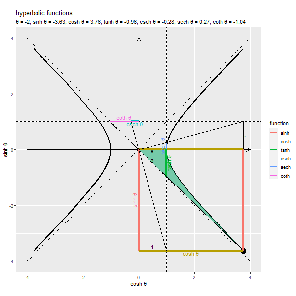
続いて、変数の値を変化させたアニメーションで確認します。
フレーム数を指定して、変数として用いる値を作成します。
# フレーム数を指定
frame_num <- 101

# 変数の値を作成
theta_i <- seq(from = -2, to = 2, length.out = frame_num) # 範囲を指定
head(theta_i)
## [1] -2.00 -1.96 -1.92 -1.88 -1.84 -1.80
フレーム数frame_numを指定して、frame_num個の$\theta$の値を作成します。
・作図コード(クリックで展開)
フレーム切替用のラベルとして使う文字列ベクトルを作成します。
# フレーム切替用ラベルのレベルを作成
frame_label_vec <- paste0(
  "θ = ", round(theta_i, digits = 2),
  ", sinh θ = ", round(sinh(theta_i), digits = 2),
  ", cosh θ = ", round(cosh(theta_i), digits = 2),
  ", tanh θ = ", round(tanh(theta_i), digits = 2),
  ", csch θ = ", round(1/sinh(theta_i), digits = 2),
  ", sech θ = ", round(1/cosh(theta_i), digits = 2),
  ", coth θ = ", round(1/tanh(theta_i), digits = 2)
)
head(frame_label_vec)
## [1] "θ = -2, sinh θ = -3.63, cosh θ = 3.76, tanh θ = -0.96, csch θ = -0.28, sech θ = 0.27, coth θ = -1.04"
## [2] "θ = -1.96, sinh θ = -3.48, cosh θ = 3.62, tanh θ = -0.96, csch θ = -0.29, sech θ = 0.28, coth θ = -1.04"
## [3] "θ = -1.92, sinh θ = -3.34, cosh θ = 3.48, tanh θ = -0.96, csch θ = -0.3, sech θ = 0.29, coth θ = -1.04"
## [4] "θ = -1.88, sinh θ = -3.2, cosh θ = 3.35, tanh θ = -0.95, csch θ = -0.31, sech θ = 0.3, coth θ = -1.05"
## [5] "θ = -1.84, sinh θ = -3.07, cosh θ = 3.23, tanh θ = -0.95, csch θ = -0.33, sech θ = 0.31, coth θ = -1.05"
## [6] "θ = -1.8, sinh θ = -2.94, cosh θ = 3.11, tanh θ = -0.95, csch θ = -0.34, sech θ = 0.32, coth θ = -1.06"
この例では、変数と関数の値をグラフに表示するために、フレームごとの値をフレーム切替用のラベル列として使います。
theta_iの値と対応する関数の値を文字列結合します。
曲線上の点を描画するためのデータフレームを作成します。
# 曲線上の点の描画用
anim_point_df <- tibble::tibble(
  t = theta_i,
  x = cosh(theta_i),
  y = sinh(theta_i),
  frame_label = factor(frame_label_vec, levels = frame_label_vec) # フレーム切替用ラベル
)
anim_point_df
## # A tibble: 101 × 4
##        t     x     y frame_label
##    <dbl> <dbl> <dbl> <fct>
##  1 -2     3.76 -3.63 θ = -2, sinh θ = -3.63, cosh θ = 3.76, tanh θ = -0.96,…
##  2 -1.96  3.62 -3.48 θ = -1.96, sinh θ = -3.48, cosh θ = 3.62, tanh θ = -0.…
##  3 -1.92  3.48 -3.34 θ = -1.92, sinh θ = -3.34, cosh θ = 3.48, tanh θ = -0.…
##  4 -1.88  3.35 -3.20 θ = -1.88, sinh θ = -3.2, cosh θ = 3.35, tanh θ = -0.9…
##  5 -1.84  3.23 -3.07 θ = -1.84, sinh θ = -3.07, cosh θ = 3.23, tanh θ = -0.…
##  6 -1.8   3.11 -2.94 θ = -1.8, sinh θ = -2.94, cosh θ = 3.11, tanh θ = -0.9…
##  7 -1.76  2.99 -2.82 θ = -1.76, sinh θ = -2.82, cosh θ = 2.99, tanh θ = -0.…
##  8 -1.72  2.88 -2.70 θ = -1.72, sinh θ = -2.7, cosh θ = 2.88, tanh θ = -0.9…
##  9 -1.68  2.78 -2.59 θ = -1.68, sinh θ = -2.59, cosh θ = 2.78, tanh θ = -0.…
## 10 -1.64  2.67 -2.48 θ = -1.64, sinh θ = -2.48, cosh θ = 2.67, tanh θ = -0.…
## # … with 91 more rows
変数$\theta$と関数$\cosh \theta, \sinh \theta$の値をフレーム切替用のラベルとあわせて格納します。
変数の値(の半分)を面積(塗りつぶし領域)として描画するためのデータフレームを作成します。
# 変数(面積)の描画用
anim_variable_area_df <- tibble::tibble(
  t = theta_i,
  frame_label = factor(frame_label_vec, levels = frame_label_vec) # フレーム切替用ラベル
) |>
  dplyr::group_by(t, frame_label) |> # x軸の値の作成用
  dplyr::summarise(
    x = seq(from = 0, to = cosh(t), length.out = 50), .groups = "drop"
  ) |> # フレームごとにx軸の値を作成
  dplyr::mutate(
    sign = dplyr::if_else(t >= 0, true = 1, false = -1), # 符号
    curve = sign * sqrt(x^2 - 1), # x軸と双曲線上の線分
    curve = dplyr::if_else(is.na(curve), true = 0, false = curve), # 双曲線の範囲外を0に置換
    straight = sinh(t)/cosh(t) * x # 原点と曲線上の点の線分
  )
anim_variable_area_df
## # A tibble: 5,050 × 6
##        t frame_label                                   x  sign curve straight
##    <dbl> <fct>                                     <dbl> <dbl> <dbl>    <dbl>
##  1    -2 θ = -2, sinh θ = -3.63, cosh θ = 3.76, … 0         -1     0   0
##  2    -2 θ = -2, sinh θ = -3.63, cosh θ = 3.76, … 0.0768    -1     0  -0.0740
##  3    -2 θ = -2, sinh θ = -3.63, cosh θ = 3.76, … 0.154     -1     0  -0.148
##  4    -2 θ = -2, sinh θ = -3.63, cosh θ = 3.76, … 0.230     -1     0  -0.222
##  5    -2 θ = -2, sinh θ = -3.63, cosh θ = 3.76, … 0.307     -1     0  -0.296
##  6    -2 θ = -2, sinh θ = -3.63, cosh θ = 3.76, … 0.384     -1     0  -0.370
##  7    -2 θ = -2, sinh θ = -3.63, cosh θ = 3.76, … 0.461     -1     0  -0.444
##  8    -2 θ = -2, sinh θ = -3.63, cosh θ = 3.76, … 0.537     -1     0  -0.518
##  9    -2 θ = -2, sinh θ = -3.63, cosh θ = 3.76, … 0.614     -1     0  -0.592
## 10    -2 θ = -2, sinh θ = -3.63, cosh θ = 3.76, … 0.691     -1     0  -0.666
## # … with 5,040 more rows
変数の値とフレーム切替用のラベルを格納して、変数の値(フレーム)ごとに(t, frame_label列でグループ化して)、塗りつぶし範囲の曲線と直線(下限と上限)の値を計算します。
変数の値に応じてx軸の範囲($0 \leq x \leq \cosh \theta$)が変わるので、フレームごとにsummarise()でx列の値を作成して計算に使います。
変数ラベルを描画するためのデータフレームを作成します。
# 変数ラベルの描画用
anim_variable_label_df <- tibble::tibble(
  t = theta_i,
  x = 0.5,
  y = 0.25 * tanh(theta_i),
  frame_label = factor(frame_label_vec, levels = frame_label_vec) # フレーム切替用ラベル
)
anim_variable_label_df
## # A tibble: 101 × 4
##        t     x      y frame_label
##    <dbl> <dbl>  <dbl> <fct>
##  1 -2      0.5 -0.241 θ = -2, sinh θ = -3.63, cosh θ = 3.76, tanh θ = -0.96…
##  2 -1.96   0.5 -0.240 θ = -1.96, sinh θ = -3.48, cosh θ = 3.62, tanh θ = -0…
##  3 -1.92   0.5 -0.239 θ = -1.92, sinh θ = -3.34, cosh θ = 3.48, tanh θ = -0…
##  4 -1.88   0.5 -0.239 θ = -1.88, sinh θ = -3.2, cosh θ = 3.35, tanh θ = -0.…
##  5 -1.84   0.5 -0.238 θ = -1.84, sinh θ = -3.07, cosh θ = 3.23, tanh θ = -0…
##  6 -1.8    0.5 -0.237 θ = -1.8, sinh θ = -2.94, cosh θ = 3.11, tanh θ = -0.…
##  7 -1.76   0.5 -0.236 θ = -1.76, sinh θ = -2.82, cosh θ = 2.99, tanh θ = -0…
##  8 -1.72   0.5 -0.234 θ = -1.72, sinh θ = -2.7, cosh θ = 2.88, tanh θ = -0.…
##  9 -1.68   0.5 -0.233 θ = -1.68, sinh θ = -2.59, cosh θ = 2.78, tanh θ = -0…
## 10 -1.64   0.5 -0.232 θ = -1.64, sinh θ = -2.48, cosh θ = 2.67, tanh θ = -0…
## # … with 91 more rows
この例では、$x = 0.5$の位置に変数ラベルを配置します。塗りつぶし範囲のy軸の中点は$\frac{x \tanh \theta}{2}$で計算できます。
双曲線関数を直線として描画するためのデータフレームを作成します。
# 双曲線関数直線の描画用
anim_function_line_df <- tibble::tibble(
  x_from = c(
    rep(0, times = frame_num), cosh(theta_i),
    rep(0, times = frame_num), rep(0, times = frame_num),
    rep(1, times = frame_num),
    rep(0, times = frame_num), rep(1, times = frame_num), rep(0, times = frame_num)
  ),
  y_from = c(
    rep(0, times = frame_num), rep(0, times = frame_num),
    rep(0, times = frame_num), sinh(theta_i),
    rep(0, times = frame_num),
    rep(1, times = frame_num), rep(0, times = frame_num), rep(1, times = frame_num)
  ),
  x_to = c(
    rep(0, times = frame_num), cosh(theta_i),
    cosh(theta_i), cosh(theta_i),
    rep(1, times = frame_num),
    1/sinh(theta_i), rep(1, times = frame_num), 1/tanh(theta_i)
  ),
  y_to = c(
    sinh(theta_i), sinh(theta_i),
    rep(0, times = frame_num), sinh(theta_i),
    tanh(theta_i),
    rep(1, times = frame_num), 1/cosh(theta_i), rep(1, times = frame_num)
  ),
  fnc = c(
    "sinh", "sinh",
    "cosh", "cosh",
    "tanh",
    "csch", "sech", "coth"
  ) |>
    rep(each = frame_num) |>
    factor(levels = fnc_level_vec), # 色分け用
  label_flag = c(
    TRUE, FALSE,
    FALSE, TRUE,
    TRUE,
    TRUE, TRUE, TRUE
  ) |>
    rep(each = frame_num), # 関数ラベル用
  frame_label = frame_label_vec |>
    rep(times = 8) |>
    factor(levels = frame_label_vec) # フレーム切替用ラベル
)
anim_function_line_df
## # A tibble: 808 × 7
##    x_from y_from  x_to  y_to fnc   label_flag frame_label
##     <dbl>  <dbl> <dbl> <dbl> <fct> <lgl>      <fct>
##  1      0      0     0 -3.63 sinh  TRUE       θ = -2, sinh θ = -3.63, cosh θ…
##  2      0      0     0 -3.48 sinh  TRUE       θ = -1.96, sinh θ = -3.48, cosh…
##  3      0      0     0 -3.34 sinh  TRUE       θ = -1.92, sinh θ = -3.34, cosh…
##  4      0      0     0 -3.20 sinh  TRUE       θ = -1.88, sinh θ = -3.2, cosh …
##  5      0      0     0 -3.07 sinh  TRUE       θ = -1.84, sinh θ = -3.07, cosh…
##  6      0      0     0 -2.94 sinh  TRUE       θ = -1.8, sinh θ = -2.94, cosh …
##  7      0      0     0 -2.82 sinh  TRUE       θ = -1.76, sinh θ = -2.82, cosh…
##  8      0      0     0 -2.70 sinh  TRUE       θ = -1.72, sinh θ = -2.7, cosh …
##  9      0      0     0 -2.59 sinh  TRUE       θ = -1.68, sinh θ = -2.59, cosh…
## 10      0      0     0 -2.48 sinh  TRUE       θ = -1.64, sinh θ = -2.48, cosh…
## # … with 798 more rows
「グラフの作成」と同様に、frame_num個の座標を格納します。
関数名をラベルとして描画するためのデータフレームを作成します。
# 双曲線関数ラベルの描画用
anim_function_label_df <- anim_function_line_df |>
  dplyr::filter(label_flag) |> # ラベル付けする辺を抽出
  dplyr::group_by(fnc, frame_label) |> # 中点の計算用
  dplyr::summarise(
    x = median(c(x_from, x_to)),
    y = median(c(y_from, y_to)), .groups = "drop"
  ) |>
  tibble::add_column(
    angle = c(90, 0, 90, 0, 90, 0) |>
      rep(each = frame_num),
    v = c(-0.5, 1, 1, 1, -0.5, -0.5) |>
      rep(each = frame_num),
    fnc_label = c("sinh~theta", "cosh~theta", "tanh~theta", "csch~theta", "sech~theta", "coth~theta") |>
      rep(each = frame_num) # 関数ラベル
  )
anim_function_label_df
## # A tibble: 606 × 7
##    fnc   frame_label                            x     y angle     v fnc_label
##    <fct> <fct>                              <dbl> <dbl> <dbl> <dbl> <chr>
##  1 sinh  θ = -2, sinh θ = -3.63, cosh θ = …     0 -1.81    90  -0.5 sinh~theta
##  2 sinh  θ = -1.96, sinh θ = -3.48, cosh θ…     0 -1.74    90  -0.5 sinh~theta
##  3 sinh  θ = -1.92, sinh θ = -3.34, cosh θ…     0 -1.67    90  -0.5 sinh~theta
##  4 sinh  θ = -1.88, sinh θ = -3.2, cosh θ …     0 -1.60    90  -0.5 sinh~theta
##  5 sinh  θ = -1.84, sinh θ = -3.07, cosh θ…     0 -1.53    90  -0.5 sinh~theta
##  6 sinh  θ = -1.8, sinh θ = -2.94, cosh θ …     0 -1.47    90  -0.5 sinh~theta
##  7 sinh  θ = -1.76, sinh θ = -2.82, cosh θ…     0 -1.41    90  -0.5 sinh~theta
##  8 sinh  θ = -1.72, sinh θ = -2.7, cosh θ …     0 -1.35    90  -0.5 sinh~theta
##  9 sinh  θ = -1.68, sinh θ = -2.59, cosh θ…     0 -1.29    90  -0.5 sinh~theta
## 10 sinh  θ = -1.64, sinh θ = -2.48, cosh θ…     0 -1.24    90  -0.5 sinh~theta
## # … with 596 more rows
flag_label列がTRUEの列を取り出して、関数とフレームごとに(fnc, frame_label列でグループ化して)、中点の座標をmedian()で計算します。
導出に利用する補助線を描画するためのデータフレームを作成します。
# 補助線の描画用
anim_sub_line_df <- tibble::tibble(
  x_from = c(
    apply(cbind(0, 1/sinh(theta_i)), MARGIN = 1, FUN = min),
    rep(0, times = frame_num),
    apply(cbind(0, 1/tanh(theta_i)), MARGIN = 1, FUN = min),
    rep(0, times = frame_num), cosh(theta_i)
  ),
  y_from = c(
    ifelse(theta_i >= 0, yes = 0, no = 1),
    rep(0, times = frame_num),
    ifelse(theta_i >= 0, yes = 0, no = 1),
    sinh(theta_i), rep(0, times = frame_num)
  ),
  x_to = c(
    apply(cbind(1, 1/sinh(theta_i)), MARGIN = 1, FUN = max),
    cosh(theta_i),
    ifelse((sinh(theta_i) > 0 & sinh(theta_i) < 1), yes = 1/tanh(theta_i), no = cosh(theta_i)),
    rep(1, times = frame_num), cosh(theta_i)
  ),
  y_to = c(
    ifelse(theta_i > 0, yes = apply(cbind(1, sinh(theta_i)), MARGIN = 1, FUN = max), no = sinh(theta_i)),
    rep(1, times = frame_num),
    ifelse((sinh(theta_i) > 0 & sinh(theta_i) < 1), yes = 1, no = sinh(theta_i)),
    sinh(theta_i), rep(1, times = frame_num)
  ),
  fnc = c(
    "csch", "sech", "coth",
    "1(csch)", "1(sech)"
  ) |>
    rep(each = frame_num), # 確認用
  frame_label = frame_label_vec |>
    rep(times = 5) |>
    factor(levels = frame_label_vec) # フレーム切替用ラベル
)
anim_sub_line_df
## # A tibble: 505 × 6
##    x_from y_from  x_to  y_to fnc   frame_label
##     <dbl>  <dbl> <dbl> <dbl> <chr> <fct>
##  1 -0.276      1     1 -3.63 csch  θ = -2, sinh θ = -3.63, cosh θ = 3.76, ta…
##  2 -0.287      1     1 -3.48 csch  θ = -1.96, sinh θ = -3.48, cosh θ = 3.62,…
##  3 -0.300      1     1 -3.34 csch  θ = -1.92, sinh θ = -3.34, cosh θ = 3.48,…
##  4 -0.312      1     1 -3.20 csch  θ = -1.88, sinh θ = -3.2, cosh θ = 3.35, …
##  5 -0.326      1     1 -3.07 csch  θ = -1.84, sinh θ = -3.07, cosh θ = 3.23,…
##  6 -0.340      1     1 -2.94 csch  θ = -1.8, sinh θ = -2.94, cosh θ = 3.11, …
##  7 -0.355      1     1 -2.82 csch  θ = -1.76, sinh θ = -2.82, cosh θ = 2.99,…
##  8 -0.370      1     1 -2.70 csch  θ = -1.72, sinh θ = -2.7, cosh θ = 2.88, …
##  9 -0.386      1     1 -2.59 csch  θ = -1.68, sinh θ = -2.59, cosh θ = 2.78,…
## 10 -0.403      1     1 -2.48 csch  θ = -1.64, sinh θ = -2.48, cosh θ = 2.67,…
## # … with 495 more rows
「グラフの作成」と同様に、frame_num個の座標を格納します。
定数ラベルを描画するためのデータフレームを作成します。
# 定数ラベルの描画用
anim_constant_label_df <- tibble::tibble(
  x = c(rep(0.5, times = frame_num), cosh(theta_i)),
  y = c(sinh(theta_i), rep(0.5, times = frame_num)),
  angle = c(0, 90) |>
    rep(each = frame_num),
  v = c(-0.5, 1) |>
    rep(each = frame_num),
  fnc_label = c("1", "1") |>
    rep(each = frame_num), # 関数ラベル
  frame_label = frame_label_vec |>
    rep(times = 2) |>
    factor(levels = frame_label_vec) # フレーム切替用ラベル
)
anim_constant_label_df
## # A tibble: 202 × 6
##        x     y angle     v fnc_label frame_label
##    <dbl> <dbl> <dbl> <dbl> <chr>     <fct>
##  1   0.5 -3.63     0  -0.5 1         θ = -2, sinh θ = -3.63, cosh θ = 3.76, …
##  2   0.5 -3.48     0  -0.5 1         θ = -1.96, sinh θ = -3.48, cosh θ = 3.6…
##  3   0.5 -3.34     0  -0.5 1         θ = -1.92, sinh θ = -3.34, cosh θ = 3.4…
##  4   0.5 -3.20     0  -0.5 1         θ = -1.88, sinh θ = -3.2, cosh θ = 3.35…
##  5   0.5 -3.07     0  -0.5 1         θ = -1.84, sinh θ = -3.07, cosh θ = 3.2…
##  6   0.5 -2.94     0  -0.5 1         θ = -1.8, sinh θ = -2.94, cosh θ = 3.11…
##  7   0.5 -2.82     0  -0.5 1         θ = -1.76, sinh θ = -2.82, cosh θ = 2.9…
##  8   0.5 -2.70     0  -0.5 1         θ = -1.72, sinh θ = -2.7, cosh θ = 2.88…
##  9   0.5 -2.59     0  -0.5 1         θ = -1.68, sinh θ = -2.59, cosh θ = 2.7…
## 10   0.5 -2.48     0  -0.5 1         θ = -1.64, sinh θ = -2.48, cosh θ = 2.6…
## # … with 192 more rows
「グラフの作成」と同様に、frame_num個の座標を格納します。
単位双曲線上の双曲線関数のアニメーションを作成します。
# 双曲線関数のアニメーションを作図
anim <- ggplot() +
  geom_segment(data = axis_df,
               mapping = aes(x = x_from, y = y_from, xend = x_to, yend = y_to, group = "axis"),
               arrow = arrow(length = unit(10, units = "pt"))) + # 軸線
  geom_line(data = asymptote_df,
            mapping = aes(x = x, y = y, group = slope),
            linetype = "dashed") + # 漸近線
  geom_hline(yintercept = 1, linetype = "dashed") + # csch,coth関数用の補助線
  geom_vline(xintercept = 1, linetype = "dashed") + # tanh,sech関数用の補助線
  geom_path(data = hyperbola_df,
            mapping = aes(x = cosh_t, y = sinh_t, group = sign),
            size = 1) + # 双曲線
  geom_point(data = anim_point_df,
             mapping = aes(x = x, y = y),
             size = 5) + # 双曲線上の点
  geom_ribbon(data = anim_variable_area_df,
              mapping = aes(x = x, ymin = curve, ymax = straight),
              fill = "#00A968", alpha = 0.5) + # 変数(面積)
  geom_text(mapping = aes(x = 0.5, y = 0.25*tanh(theta), label = "frac(theta, 2)"), parse = TRUE,
            size = 3) + # 変数ラベル
  geom_segment(data = anim_function_line_df,
               mapping = aes(x = x_from, y = y_from, xend = x_to, yend = y_to,
                             color = fnc, size = fnc)) + # 双曲線関数直線
  geom_segment(data = anim_sub_line_df,
               mapping = aes(x = x_from, y = y_from, xend = x_to, yend = y_to)) + # 導出用の辺
  geom_text(data = anim_constant_label_df,
            mapping = aes(x = x, y = y, label = fnc_label, angle = angle, vjust = v)) + # 定数ラベル
  geom_text(data = anim_function_label_df,
            mapping = aes(x = x, y = y, label = fnc_label,
                          color = fnc, angle = angle, vjust = v), parse = TRUE,
            show.legend = FALSE) + # 双曲線関数ラベル
  gganimate::transition_manual(frames = frame_label) + # フレーム
  scale_color_manual(breaks = fnc_level_vec,
                     values = scales::hue_pal()(length(fnc_level_vec))) +
  scale_size_manual(breaks = c("sinh", "cosh", "tanh", "csch", "sech", "coth"),
                    values = c(1.5, 1.5, 1.5, 1.5, 1, 1), guide = "none") +
  coord_fixed(ratio = 1,
              xlim = c(-axis_max, axis_max), ylim = c(-axis_max, axis_max)) + # 表示範囲
  labs(title = "hyperbolic functions",
       subtitle = "{current_frame}",
       color = "function",
       x = expression(cosh~theta), y = expression(sinh~theta))

# gif画像を作成
gganimate::animate(plot = anim, nframes = frame_num, fps = 10, width = 600, height = 600)
gganimateパッケージを利用して、アニメーション(gif画像)を作成します。
transition_manual()のフレーム制御の引数framesにフレーム(変数)ラベル列frame_labelを指定して、グラフを作成します。
animate()のplot引数にグラフオブジェクト、nframes引数にフレーム数frame_numを指定して、gif画像を作成します。また、fps引数に1秒当たりのフレーム数を指定できます。
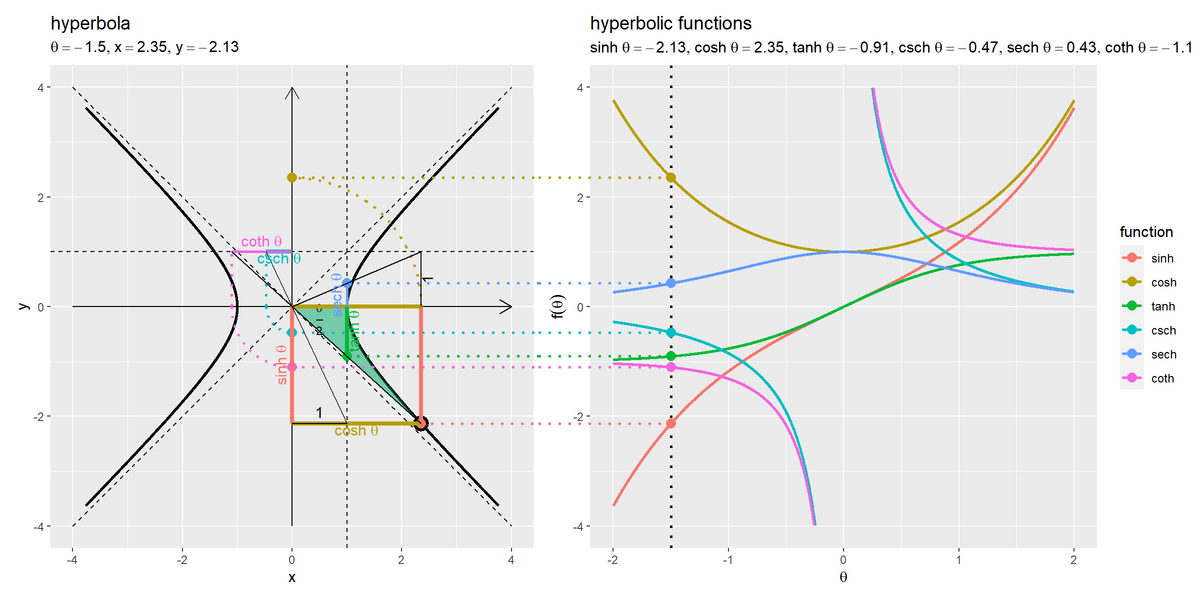
双曲線上の点と各双曲線関数曲線の関係の可視化
最後は、双曲線上における各双曲線関数の値(直線)と、各双曲線関数の曲線の関係をグラフで確認します。
グラフの作成
変数を固定したグラフで確認します。
・作図コード(クリックで展開)
双曲線関数を直線として描画するためのデータフレームを作成します。
# 双曲線関数直線の描画用
function_line_df <- tibble::tibble(
  x_from = c(
    0, cosh(theta), 0, 0, 1,
    0, 1/sinh(theta), 1, 0, 1/tanh(theta)
  ),
  y_from = c(
    0, 0, 0, sinh(theta), 0,
    1, 0, 0, 1, 0
  ),
  x_to = c(
    0, cosh(theta), cosh(theta), cosh(theta), 1,
    1/sinh(theta), 1/sinh(theta), 1, 1/tanh(theta), 1/tanh(theta)
  ),
  y_to = c(
    sinh(theta), sinh(theta), 0, sinh(theta), tanh(theta),
    1, 1, 1/cosh(theta), 1, 1
  ),
  fnc = c(
    "sinh", "sinh", "cosh", "cosh", "tanh",
    "csch", "csch", "sech", "coth", "coth"
  ) |>
    factor(levels = fnc_level_vec), # 色分け用
  label_flag = c(
    TRUE, FALSE, FALSE, TRUE, TRUE,
    TRUE, FALSE, TRUE, TRUE, FALSE
  ), # 関数ラベル用
  line_type = c(
    "main", "main", "main", "main", "main",
    "main", "sub", "main", "main", "sub"
  ), # 線の種類用
  line_width = c(
    "bold", "bold", "bold", "bold", "bold",
    "bold", "normal", "normal", "normal", "normal"
  )
)
function_line_df
## # A tibble: 10 × 8
##    x_from y_from   x_to   y_to fnc   label_flag line_type line_width
##     <dbl>  <dbl>  <dbl>  <dbl> <fct> <lgl>      <chr>     <chr>
##  1  0       0     0     -2.13  sinh  TRUE       main      bold
##  2  2.35    0     2.35  -2.13  sinh  FALSE      main      bold
##  3  0       0     2.35   0     cosh  FALSE      main      bold
##  4  0      -2.13  2.35  -2.13  cosh  TRUE       main      bold
##  5  1       0     1     -0.905 tanh  TRUE       main      bold
##  6  0       1    -0.470  1     csch  TRUE       main      bold
##  7 -0.470   0    -0.470  1     csch  FALSE      sub       normal
##  8  1       0     1      0.425 sech  TRUE       main      normal
##  9  0       1    -1.10   1     coth  TRUE       main      normal
## 10 -1.10    0    -1.10   1     coth  FALSE      sub       normal
「双曲線上の双曲線関数の可視化」のときの座標に、x軸線上への平行移動を示す補助線の座標を追加します。
また、関数直線と補助線を区別するためのline_type列と、線が重なっても上手く表示されるように制御するためのline_width列を追加します。
90度回転させる軌道を描画するためのデータフレームを作成します。
# 軸変換線の描画用
adapt_df <- dplyr::bind_rows(
  tibble::tibble(
    t = seq(from = 0, to = 0.5*pi, length.out = 100),
    x = cos(t) * cosh(theta),
    y = sin(t) * cosh(theta),
    fnc = factor("cosh", levels = fnc_level_vec) # 色分け用
  ),
  tibble::tibble(
    t = dplyr::case_when(
      theta < 0 ~ seq(from = pi, to = 1.5*pi, length.out = 100),
      theta == 0 ~ 0,
      theta > 0 ~ seq(from = 0, to = 0.5*pi, length.out = 100)
    ),
    x = cos(t) / abs(sinh(theta)),
    y = sin(t) / abs(sinh(theta)),
    fnc = factor("csch", levels = fnc_level_vec) # 色分け用
  ),
  tibble::tibble(
    t = dplyr::case_when(
      theta < 0 ~ seq(from = pi, to = 1.5*pi, length.out = 100),
      theta == 0 ~ 0,
      theta > 0 ~ seq(from = 0, to = 0.5*pi, length.out = 100)
    ),
    x = cos(t) / abs(tanh(theta)),
    y = sin(t) / abs(tanh(theta)),
    fnc = factor("coth", levels = fnc_level_vec) # 色分け用
  )
)
adapt_df
## # A tibble: 300 × 4
##         t     x      y fnc
##     <dbl> <dbl>  <dbl> <fct>
##  1 0       2.35 0      cosh
##  2 0.0159  2.35 0.0373 cosh
##  3 0.0317  2.35 0.0746 cosh
##  4 0.0476  2.35 0.112  cosh
##  5 0.0635  2.35 0.149  cosh
##  6 0.0793  2.35 0.186  cosh
##  7 0.0952  2.34 0.224  cosh
##  8 0.111   2.34 0.261  cosh
##  9 0.127   2.33 0.298  cosh
## 10 0.143   2.33 0.335  cosh
## # … with 290 more rows
横方向に伸びる線分について、関数曲線と対応させるために90度回転させる線を格納する。
弧度法における角度を作成して、半径が$f(\theta)$の絶対値の弧(原点からの長さが$|f(\theta)|$の点)の座標を計算します。$\theta > 0$のときは$0 \leq t \leq \frac{\pi}{2}$、$\theta = 0$のときは$t = 0$、$\theta < 0$のときは$\pi \leq t \leq \frac{3 \pi}{2}$の角度を使います。ただし、cosh関数については、正の値のみをとるので、$0 \leq t \leq \frac{\pi}{2}$を使います。$\theta$が正の値のときの$t$は度数法における$0^{\circ}$から$90^{\circ}$の角度、$\theta$が$0$のときは$0^{\circ}$、$\theta$が負の値のときは$180^{\circ}$から$270^{\circ}$の角度に対応します。
半径が$a$の円のx軸の値は$x = a \cos t$、y軸の値は$y = a \sin t$で計算できます。
絶対値はabs()で計算できます。
双曲線関数直線(双曲線のグラフ)上の点と双曲線関数曲線上の点を結ぶ補助線(の半分)を描画するためのデータフレームを作成します。
# 双曲線関数曲線との対応用
l <- 0.6
hyperbola_segment_df <- tibble::tibble(
  x_from = c(cosh(theta), 0, 1, 0, 1, 0),
  x_to = axis_max+l,
  y = c(sinh(theta), cosh(theta), tanh(theta), 1/sinh(theta), 1/cosh(theta), 1/tanh(theta)),
  fnc = c("sinh", "cosh", "tanh", "csch", "sech", "coth") |>
    factor(levels = fnc_level_vec) # 色分け用
)
hyperbola_segment_df
## # A tibble: 6 × 4
##   x_from  x_to      y fnc
##    <dbl> <dbl>  <dbl> <fct>
## 1   2.35   4.6 -2.13  sinh
## 2   0      4.6  2.35  cosh
## 3   1      4.6 -0.905 tanh
## 4   0      4.6 -0.470 csch
## 5   1      4.6  0.425 sech
## 6   0      4.6 -1.10  coth
各関数直線の先端の点または移動した点からy軸の反対側への垂線を引くように座標を指定します。
双曲線のグラフを作成します。
# 変数ラベルの描画用
hyperbola_label <- paste0(
  "list(",
  "theta==", theta,
  ", x==", round(cosh(theta), digits = 2),
  ", y==", round(sinh(theta), digits = 2),
  ")"
)

# 双曲線関数を作図
hyperbola_graph <- ggplot() +
  geom_segment(data = axis_df,
               mapping = aes(x = x_from, y = y_from, xend = x_to, yend = y_to, group = "axis"),
               arrow = arrow(length = unit(10, units = "pt"))) + # 軸線
  geom_line(data = asymptote_df,
            mapping = aes(x = x, y = y, group = slope),
            linetype = "dashed") + # 漸近線
  geom_hline(yintercept = 1, linetype = "dashed") + # csch,coth関数用の補助線
  geom_vline(xintercept = 1, linetype = "dashed") + # tanh,sech関数用の補助線
  geom_path(data = hyperbola_df,
            mapping = aes(x = cosh_t, y = sinh_t, group = sign),
            size = 1) + # 双曲線
  geom_point(data = hyperbola_point_df,
             mapping = aes(x = x, y = y),
             size = 5) + # 双曲線上の点
  geom_ribbon(data = variable_area_df,
              mapping = aes(x = x, ymin = curve, ymax = straight),
              fill = "#00A968", alpha = 0.5) + # 変数(面積)
  geom_text(mapping = aes(x = 0.5, y = 0.25*tanh(theta), label = "frac(theta, 2)"), parse = TRUE,
            size = 3) + # 変数ラベル
  geom_path(data = adapt_df,
            mapping = aes(x = x, y = y, color = fnc),
            size = 1, linetype = "dotted", show.legend = FALSE) + # x軸からy軸への変換線
  geom_segment(data = hyperbola_segment_df,
               mapping = aes(x = x_from, y = y, xend = x_to, yend = y, color = fnc),
               size = 1, linetype = "dotted", show.legend = FALSE) + # 双曲線関数曲線との対応線
  geom_point(data = hyperbola_segment_df,
             mapping = aes(x = x_from, y = y, color = fnc),
             size = 3) + # 双曲線関数点
  geom_segment(data = function_line_df,
               mapping = aes(x = x_from, y = y_from, xend = x_to, yend = y_to,
                             color = fnc, size = line_width, linetype = line_type)) + # 双曲線関数直線
  geom_segment(data = sub_line_df,
               mapping = aes(x = x_from, y = y_from, xend = x_to, yend = y_to)) + # 導出用の辺
  geom_text(data = constant_label_df,
            mapping = aes(x = x, y = y, label = fnc_label, angle = angle, vjust = v)) + # 定数ラベル
  geom_text(data = function_label_df,
            mapping = aes(x = x, y = y, label = fnc_label,
                          color = fnc, angle = angle, vjust = v), parse = TRUE,
            show.legend = FALSE) + # 双曲線関数ラベル
  scale_color_manual(breaks = fnc_level_vec,
                     values = scales::hue_pal()(length(fnc_level_vec))) +
  scale_linetype_manual(breaks = c("main", "sub"),
                        values = c("solid", "dotted"), guide = "none") +
  scale_size_manual(breaks = c("bold", "normal"),
                    values = c(1.5, 1), guide = "none") +
  coord_fixed(ratio = 1, clip = "off",
              xlim = c(-axis_max, axis_max), ylim = c(-axis_max, axis_max)) + # 表示範囲
  theme(legend.position = "none") + # 凡例を非表示
  labs(title = "hyperbola",
       subtitle = parse(text = hyperbola_label),
       color = "function",
       x = "x", y = "y")
hyperbola_graph
双曲線関数曲線上の点を描画するためのデータフレームを作成します。
# 双曲線関数上の点の描画用
function_point_df <- tibble::tibble(
  t = theta,
  f_t = c(
    sinh(theta), cosh(theta), tanh(theta),
    1/sinh(theta), 1/cosh(theta), 1/tanh(theta)
  ),
  fnc = c("sinh", "cosh", "tanh", "csch", "sech", "coth") |>
    factor(levels = fnc_level_vec) # 色分け用
)
function_point_df
## # A tibble: 6 × 3
##       t    f_t fnc
##   <dbl>  <dbl> <fct>
## 1  -1.5 -2.13  sinh
## 2  -1.5  2.35  cosh
## 3  -1.5 -0.905 tanh
## 4  -1.5 -0.470 csch
## 5  -1.5  0.425 sech
## 6  -1.5 -1.10  coth
$\theta$と各関数の値をデータフレームに格納します。
双曲線関数曲線上の点と双曲線グラフ上の点を結ぶ補助線(の半分)を描画するためのデータフレームを作成します。
# 双曲線との対応用
d <- 1.1
l <- 0.65
function_segment_df <- function_point_df |>
  dplyr::mutate(x_to = min(theta_vec)-l) |>
  dplyr::select(x_from = t, x_to, y = f_t, fnc)
function_segment_df
## # A tibble: 6 × 4
##   x_from  x_to      y fnc
##    <dbl> <dbl>  <dbl> <fct>
## 1   -1.5 -2.65 -2.13  sinh
## 2   -1.5 -2.65  2.35  cosh
## 3   -1.5 -2.65 -0.905 tanh
## 4   -1.5 -2.65 -0.470 csch
## 5   -1.5 -2.65  0.425 sech
## 6   -1.5 -2.65 -1.10  coth
曲線上の点からx軸とy軸への垂線を引くように座標を指定します。
双曲線関数のグラフを作成します。
# 双曲線関数曲線の描画用
function_curve_df <- tibble::tibble(
  t = rep(theta_vec, times = 6),
  f_t = c(
    sinh(theta_vec), cosh(theta_vec), tanh(theta_vec),
    1/sinh(theta_vec), 1/cosh(theta_vec), 1/tanh(theta_vec)
  ),
  fnc = c("sinh", "cosh", "tanh", "csch", "sech", "coth") |>
    rep(each = length(theta_vec)) |>
    factor(levels = fnc_level_vec), # 色分け用
) |>
  dplyr::mutate(
    f_t = dplyr::if_else(
      (f_t >= -axis_max & f_t <= axis_max), true = f_t, false = as.numeric(NA)
    )
  ) # 描画範囲外を欠損値に置換

# 関数ラベルの描画用
function_label <- paste0(
  "list(",
  "sinh~theta==", round(sinh(theta), digits = 2),
  ", cosh~theta==", round(cosh(theta), digits = 2),
  ", tanh~theta==", round(tanh(theta), digits = 2),
  ", csch~theta==", round(1/sinh(theta), digits = 2),
  ", sech~theta==", round(1/cosh(theta), digits = 2),
  ", coth~theta==", round(1/tanh(theta), digits = 2),
  ")"
)

# 双曲線関数曲線の作図
function_graph <- ggplot() +
  geom_vline(xintercept = theta, size = 1, linetype = "dotted") +
  geom_line(data = function_curve_df,
            mapping = aes(x = t, y = f_t, color = fnc),
            size = 1) + # 双曲線関数曲線
  geom_segment(data = function_segment_df,
               mapping = aes(x = x_from, y = y, xend = x_to, yend = y, color = fnc),
               size = 1, linetype = "dotted") + # 双曲線との対応線
  geom_point(data = function_point_df,
             mapping = aes(x = t, y = f_t, color = fnc),
             size = 3) + # 双曲線関数曲線上の点
  scale_color_manual(breaks = fnc_level_vec,
                     values = scales::hue_pal()(length(fnc_level_vec))) +
  coord_cartesian(clip = "off",
                  xlim = c(min(theta_vec), max(theta_vec)), ylim = c(-axis_max, axis_max)) + # 描画範囲
  labs(title = "hyperbolic functions",
       subtitle = parse(text = function_label),
       color = "function",
       x = expression(theta), y = expression(f(theta)))
function_graph
2つのグラフを並べて描画します。
# 並べて描画
patchwork::wrap_plots(hyperbola_graph, function_graph, guides = "collect")
patchworkパッケージのwrap_plots()を使ってグラフを並べます。
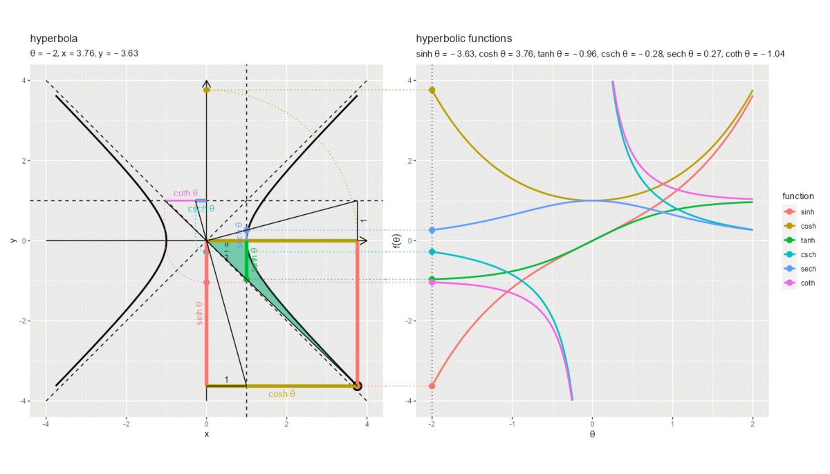
アニメーションの作成
続いて、変数の値を変化させたアニメーションで確認します。
フレーム数を指定して、変数として用いる値を作成します。
# フレーム数を指定
frame_num <- 101

# 変数の値を作成
theta_i <- seq(from = -2, to = 2, length.out = frame_num) # 範囲を指定
head(theta_i)
## [1] -2.00 -1.96 -1.92 -1.88 -1.84 -1.80
フレーム数frame_numを指定して、frame_num個の$\theta$の値を作成します。
・作図コード(クリックで展開)
theta_iから順番に値を取り出して作図し、グラフを書き出します。
# 一時保存フォルダを指定
dir_path <- "tmp_folder"

# 関数ラベルのレベルを指定
fnc_level_vec <- c("sinh", "cosh", "tanh", "csch", "sech", "coth")

# 変数ごとに作図
for(i in 1:frame_num) {

  # i番目の値を取得
  theta <- theta_i[i]

  # 双曲線上の点の描画用
  hyperbola_point_df <- tibble::tibble(
    t = theta,
    x = cosh(theta),
    y = sinh(theta),
  )

  # 変数(面積)の描画用
  variable_area_df <- tibble::tibble(
    x = seq(from = 0, to = cosh(theta), length.out = 50),
    sign = dplyr::if_else(theta >= 0, true = 1, false = -1), # 符号
    curve = sign * sqrt(x^2 - 1), # x軸と双曲線上の線分
    straight = sinh(theta)/cosh(theta) * x # 原点と曲線上の点の線分
  ) |>
    dplyr::mutate(
      curve = dplyr::if_else(is.na(curve), true = 0, false = curve)
    ) # 双曲線の範囲外を0に置換

  # 双曲線関数直線の描画用
  function_line_df <- tibble::tibble(
    tmp_x_from = c(
      0, cosh(theta), 0, 0, 1,
      0, 1/sinh(theta), 1, 0, 1/tanh(theta)
    ),
    y_from = c(
      0, 0, 0, sinh(theta), 0,
      1, 0, 0, 1, 0
    ),
    tmp_x_to = c(
      0, cosh(theta), cosh(theta), cosh(theta), 1,
      1/sinh(theta), 1/sinh(theta), 1, 1/tanh(theta), 1/tanh(theta)
    ),
    tmp_y_to = c(
      sinh(theta), sinh(theta), 0, sinh(theta), tanh(theta),
      1, 1, 1/cosh(theta), 1, 1
    ),
    fnc = c(
      "sinh", "sinh", "cosh", "cosh", "tanh",
      "csch", "csch", "sech", "coth", "coth"
    ) |>
      factor(levels = fnc_level_vec), # 色分け用
    label_flag = c(
      TRUE, FALSE, FALSE, TRUE, TRUE,
      TRUE, FALSE, TRUE, TRUE, FALSE
    ), # 関数ラベル用
    line_type = c(
      "main", "main", "main", "main", "main",
      "main", "sub", "main", "main", "sub"
    ), # 線の種類用
    line_width = c(
      "bold", "bold", "bold", "bold", "bold",
      "bold", "thin", "normal", "normal", "thin"
    ) # 線の太さ用
  ) |>
    dplyr::mutate(
      x_from = dplyr::case_when(
        (tmp_x_from < -axis_max & line_type == "main") ~ -Inf,
        (tmp_x_from > axis_max & line_type == "main") ~ Inf,
        (tmp_x_from < -axis_max & line_type == "sub") ~ as.numeric(NA),
        (tmp_x_from > axis_max & line_type == "sub") ~ as.numeric(NA),
        TRUE ~ tmp_x_from
      ),
      x_to = dplyr::case_when(
        (tmp_x_to < -axis_max & line_type == "main") ~ -Inf,
        (tmp_x_to > axis_max & line_type == "main") ~ Inf,
        (tmp_x_to < -axis_max & line_type == "sub") ~ as.numeric(NA),
        (tmp_x_to > axis_max & line_type == "sub") ~ as.numeric(NA),
        TRUE ~ tmp_x_to
      ),
      y_to = dplyr::case_when(
        tmp_y_to < -axis_max ~ -Inf,
        tmp_y_to > axis_max ~ Inf,
        TRUE ~ tmp_y_to
      )
    ) # 描画範囲外を枠の最大値に置換

  # 双曲線関数ラベルの描画用
  function_label_df <- function_line_df |>
    dplyr::filter(label_flag) |>
    dplyr::group_by(fnc) |> # 中点の計算用
    dplyr::summarise(
      x = median(c(tmp_x_from, tmp_x_to)),
      y = median(c(y_from, tmp_y_to)), .groups = "drop"
    ) |>
    tibble::add_column(
      angle = c(90, 0, 90, 0, 90, 0),
      v = c(-0.5, 1.5, 1.5, 1.5, -0.5, -0.5),
      fnc_label = c("sinh~theta", "cosh~theta", "tanh~theta", "csch~theta", "sech~theta", "coth~theta") # 関数ラベル
    ) |>
    dplyr::mutate(
      x = dplyr::case_when(
        x < -axis_max ~ -Inf,
        x > axis_max ~ Inf,
        TRUE ~ x
      ),
      y_to = dplyr::case_when(
        y < -axis_max ~ -Inf,
        y > axis_max ~ Inf,
        TRUE ~ y
      )
    ) # 描画範囲外を枠の最大値に置換

  # 補助線の描画用
  sub_line_df <- tibble::tibble(
    x_from = c(
      min(0, 1/sinh(theta)), 0, min(0, 1/tanh(theta)),
      0, cosh(theta)
    ),
    y_from = c(
      ifelse(theta >= 0, yes = 0, no = 1), 0, ifelse(theta >= 0, yes = 0, no = 1),
      sinh(theta), 0
    ),
    x_to = c(
      max(1, 1/sinh(theta)),
      cosh(theta),
      ifelse((sinh(theta) > 0 & sinh(theta) < 1), yes = 1/tanh(theta), no = cosh(theta)),
      1, cosh(theta)
    ),
    y_to = c(
      ifelse(theta > 0, yes = max(1, sinh(theta)), no = sinh(theta)),
      1,
      ifelse((sinh(theta) > 0 & sinh(theta) < 1), yes = 1, no = sinh(theta)),
      sinh(theta), 1
    ),
    fnc = c(
      "csch", "sech", "coth",
      "1(csch)", "1(sech)"
    ) # 確認用
  )

  # 定数ラベルの描画用
  constant_label_df <- tibble::tibble(
    x = c(0.5, cosh(theta)),
    y = c(sinh(theta), 0.5),
    angle = c(0, 90),
    v = c(-0.5, 1.5),
    fnc_label = c("1", "1") # 関数ラベル
  )

  # 軸変換線の描画用
  adapt_df <- dplyr::bind_rows(
    tibble::tibble(
      t = seq(from = 0, to = 0.5*pi, length.out = 100),
      x = cos(t) * cosh(theta),
      y = sin(t) * cosh(theta),
      fnc = factor("cosh", levels = fnc_level_vec) # 色分け用
    ),
    tibble::tibble(
      t = dplyr::case_when(
        theta < 0 ~ seq(from = pi, to = 1.5*pi, length.out = 100),
        theta == 0 ~ 0,
        theta > 0 ~ seq(from = 0, to = 0.5*pi, length.out = 100)
      ),
      x = cos(t) / abs(sinh(theta)),
      y = sin(t) / abs(sinh(theta)),
      fnc = factor("csch", levels = fnc_level_vec) # 色分け用
    ),
    tibble::tibble(
      t = dplyr::case_when(
        theta < 0 ~ seq(from = pi, to = 1.5*pi, length.out = 100),
        theta == 0 ~ 0,
        theta > 0 ~ seq(from = 0, to = 0.5*pi, length.out = 100)
      ),
      x = cos(t) / abs(tanh(theta)),
      y = sin(t) / abs(tanh(theta)),
      fnc = factor("coth", levels = fnc_level_vec) # 色分け用
    )
  ) |>
    dplyr::mutate(
      x = dplyr::if_else(
        (x >= -axis_max & x <= axis_max), true = x, false = as.numeric(NA)
      ),
      y = dplyr::if_else(
        (y >= -axis_max & y <= axis_max), true = y, false = as.numeric(NA)
      )
    ) # 描画範囲外を欠損値に置換

  # 双曲線関数曲線との対応用
  l <- 0.6
  hyperbola_segment_df <- tibble::tibble(
    x_from = c(cosh(theta), 0, 1, 0, 1, 0),
    x_to = axis_max+l,
    y = c(sinh(theta), cosh(theta), tanh(theta), 1/sinh(theta), 1/cosh(theta), 1/tanh(theta)),
    fnc = c("sinh", "cosh", "tanh", "csch", "sech", "coth") |>
      factor(levels = fnc_level_vec) # 色分け用
  ) |>
    dplyr::mutate(
      y = dplyr::if_else(
        (y >= -axis_max & y <= axis_max), true = y, false = as.numeric(NA)
      )
    ) # 描画範囲外を欠損値に置換

  # 変数ラベルの描画用
  hyperbola_label <- paste0(
    "list(",
    "theta==", theta,
    ", x==", round(cosh(theta), digits = 2),
    ", y==", round(sinh(theta), digits = 2),
    ")"
  )

  # 双曲線関数を作図
  hyperbola_graph <- ggplot() +
    geom_segment(data = axis_df,
                 mapping = aes(x = x_from, y = y_from, xend = x_to, yend = y_to, group = "axis"),
                 arrow = arrow(length = unit(10, units = "pt"))) + # 軸線
    geom_line(data = asymptote_df,
              mapping = aes(x = x, y = y, group = slope),
              linetype = "dashed") + # 漸近線
    geom_hline(yintercept = 1, linetype = "dashed") + # csch,coth関数用の補助線
    geom_vline(xintercept = 1, linetype = "dashed") + # tanh,sech関数用の補助線
    geom_path(data = hyperbola_df,
              mapping = aes(x = cosh_t, y = sinh_t, group = sign),
              size = 1) + # 双曲線
    geom_point(data = hyperbola_point_df,
               mapping = aes(x = x, y = y),
               size = 5) + # 双曲線上の点
    geom_ribbon(data = variable_area_df,
                mapping = aes(x = x, ymin = curve, ymax = straight),
                fill = "#00A968", alpha = 0.5) + # 変数(面積)
    geom_text(mapping = aes(x = 0.5, y = 0.25*tanh(theta), label = "frac(theta, 2)"), parse = TRUE,
              size = 3) + # 変数ラベル
    geom_path(data = adapt_df,
              mapping = aes(x = x, y = y, color = fnc),
              linetype = "dotted", show.legend = FALSE) + # x軸からy軸への変換線
    geom_segment(data = hyperbola_segment_df,
                 mapping = aes(x = x_from, y = y, xend = x_to, yend = y, color = fnc),
                 linetype = "dotted", show.legend = FALSE) + # 双曲線関数曲線との対応線
    geom_point(data = hyperbola_segment_df,
               mapping = aes(x = x_from, y = y, color = fnc),
               size = 3) + # 双曲線関数点
    geom_segment(data = function_line_df,
                 mapping = aes(x = x_from, y = y_from, xend = x_to, yend = y_to,
                               color = fnc, size = line_width, linetype = line_type)) + # 双曲線関数直線
    geom_segment(data = sub_line_df,
                 mapping = aes(x = x_from, y = y_from, xend = x_to, yend = y_to)) + # 導出用の辺
    geom_text(data = constant_label_df,
              mapping = aes(x = x, y = y, label = fnc_label, angle = angle, vjust = v)) + # 定数ラベル
    geom_text(data = function_label_df,
              mapping = aes(x = x, y = y, label = fnc_label,
                            color = fnc, angle = angle, vjust = v), parse = TRUE,
              show.legend = FALSE) + # 双曲線関数ラベル
    scale_color_manual(breaks = fnc_level_vec,
                       values = scales::hue_pal()(length(fnc_level_vec))) +
    scale_linetype_manual(breaks = c("main", "sub"),
                          values = c("solid", "dotted"), guide = "none") +
    scale_size_manual(breaks = c("bold", "normal", "thin"),
                      values = c(2, 1, 0.5), guide = "none") +
    theme(legend.position = "none") + # 凡例を非表示
    coord_fixed(ratio = 1, clip = "off",
                xlim = c(-axis_max, axis_max), ylim = c(-axis_max, axis_max)) + # 表示範囲
    labs(title = "hyperbola",
         subtitle = parse(text = hyperbola_label),
         color = "function",
         x = "x", y = "y")

  # 双曲線関数上の点の描画用
  function_point_df <- tibble::tibble(
    t = theta,
    f_t = c(
      sinh(theta), cosh(theta), tanh(theta),
      1/sinh(theta), 1/cosh(theta), 1/tanh(theta)
    ),
    fnc = c("sinh", "cosh", "tanh", "csch", "sech", "coth") |>
      factor(levels = fnc_level_vec) # 色分け用
  ) |>
    dplyr::mutate(
      f_t = dplyr::if_else(
        (f_t > -axis_max & f_t <= axis_max), true = f_t, false = as.numeric(NA)
      )
    ) # 描画範囲外を欠損値に置換

  # 双曲線関数曲線の描画用
  function_curve_df <- tibble::tibble(
    t = rep(theta_vec, times = 6),
    f_t = c(
      sinh(theta_vec), cosh(theta_vec), tanh(theta_vec),
      1/sinh(theta_vec), 1/cosh(theta_vec), 1/tanh(theta_vec)
    ),
    fnc = c("sinh", "cosh", "tanh", "csch", "sech", "coth") |>
      rep(each = length(theta_vec)) |>
      factor(levels = fnc_level_vec), # 色分け用
  ) |>
    dplyr::mutate(
      f_t = dplyr::if_else(
        (f_t >= -axis_max & f_t <= axis_max), true = f_t, false = as.numeric(NA)
      )
    ) # 描画範囲外を欠損値に置換

  # 双曲線との対応用
  d <- 1.1
  l <- 0.6
  function_segment_df <- function_point_df |>
    dplyr::mutate(x_to = min(theta_vec)-l) |>
    dplyr::select(x_from = t, x_to, y = f_t, fnc)

  # 関数ラベルの描画用
  function_label <- paste0(
    "list(",
    "sinh~theta==", round(sinh(theta), digits = 2),
    ", cosh~theta==", round(cosh(theta), digits = 2),
    ", tanh~theta==", round(tanh(theta), digits = 2),
    ", csch~theta==", round(1/sinh(theta), digits = 2),
    ", sech~theta==", round(1/cosh(theta), digits = 2),
    ", coth~theta==", round(1/tanh(theta), digits = 2),
    ")"
  )

  # 双曲線関数曲線の作図
  function_graph <- ggplot() +
    geom_vline(xintercept = theta, linetype = "dotted") +
    geom_line(data = function_curve_df,
              mapping = aes(x = t, y = f_t, color = fnc),
              size = 1) + # 双曲線関数曲線
    geom_segment(data = function_segment_df,
                 mapping = aes(x = x_from, y = y, xend = x_to, yend = y, color = fnc),
                 linetype = "dotted") + # 双曲線との対応線
    geom_point(data = function_point_df,
               mapping = aes(x = t, y = f_t, color = fnc),
               size = 3) + # 双曲線関数曲線上の点
    scale_color_manual(breaks = fnc_level_vec,
                       values = scales::hue_pal()(length(fnc_level_vec))) +
    coord_cartesian(clip = "off",
                    xlim = c(min(theta_vec), max(theta_vec)), ylim = c(-axis_max, axis_max)) + # 描画範囲
    labs(title = "hyperbolic functions",
         subtitle = parse(text = function_label),
         color = "function",
         x = expression(theta), y = expression(f(theta)))

  # 並べて描画
  graph <- patchwork::wrap_plots(hyperbola_graph, function_graph, guides = "collect")

  # ファイルを書き出し
  file_path <- paste0(dir_path, "/", stringr::str_pad(i, width = nchar(frame_num), pad = "0"), ".png")
  ggplot2::ggsave(filename = file_path, plot = graph, width = 1400, height = 800, units = "px", dpi = 100)

  # 途中経過を表示
  message("\r", i, " / ", frame_num, appendLF = FALSE)
}
変数の値ごとに「グラフの作成」と同様に処理します。ただし、グラフサイズ(-axis_maxからaxis_max)外の場合は表示しないように、欠損値などに置き換える処理を追加しています。
作成したグラフをggsave()で保存します。
双曲線関数のアニメーションを作成します。
# gif画像を作成
paste0(dir_path, "/", stringr::str_pad(1:frame_num, width = nchar(frame_num), pad = "0"), ".png") |> # ファイルパスを作成
  magick::image_read() |> # 画像ファイルを読込
  magick::image_animate(fps = 1, dispose = "previous") |> # gif画像を作成
  magick::image_write_gif(path = "hyperbolic_function.gif", delay = 0.1) -> tmp_path # gifファイル書き出
全てのファイルパスを作成して、image_read()で画像ファイルを読み込んで、image_animate()でgif画像に変換して、image_write_gif()でgifファイルを書き出します。delay引数に1秒当たりのフレーム数の逆数を指定します。
この記事では、双曲線関数を可視化しました。
おわりに
これで双曲線関数の可視化シリーズは終了です。三角関数の可視化シリーズに戻りますか。
何に使われるのか未だに分かってませんが、漸近線との関係から最大値や最小値が1になるとか超える超えないとかがよく分かって面白かったです。
いつもいつも、2・3日で書けるだろうと思って書き始めて半月とかかかるんですが、今回もその例にもれずでした。もう少しなんとかならんものか。
そんなこんなでエンディングにこの曲をどうぞ♪
全部載せてDong!!