はじめに

　円関数(三角関数)の定義や性質、公式などを可視化して理解しようシリーズです。

　この記事では、arctan関数のグラフを作成します。

【前の内容】

www.anarchive-beta.com

【他の内容】

www.anarchive-beta.com

【この記事の内容】

はじめに
arctan関数の定義の可視化
おわりに

arctan関数の定義の可視化

　arctan関数(逆tan関数・逆正接関数・逆タンジェント関数・inverse tangent function)の定義をグラフで確認します。arctan関数は、逆円関数(inverse circular functions)・逆三角関数(inverse trigonometric functions)の1つです。
　tan関数の定義や作図については「【R】tan関数の可視化 - からっぽのしょこ」を参照してください。

　利用するパッケージを読み込みます。

# 利用パッケージ
library(tidyverse)

　この記事では、基本的に パッケージ名::関数名() の記法を使うので、パッケージの読み込みは不要です。ただし、作図コードについてはパッケージ名を省略するので、ggplot2 を読み込む必要があります。
　また、ネイティブパイプ演算子 |> を使います。magrittr パッケージのパイプ演算子 %>% に置き換えられますが、その場合は magrittr を読み込む必要があります。

定義式の確認

　まずは、arctan関数の定義式を確認します。

　tan関数は、sin関数とcos関数の商で定義されます。

$\displaystyle \tan x = \frac{\sin x}{\cos x}$

　arctan関数は、tan関数の逆関数で定義されます。

$\displaystyle \arctan x = \tan^{-1} x$

　定義域は $-\infty \leq x \leq \infty$ 、終域は $-\frac{\pi}{2} \lt \arctan x \lt \frac{\pi}{2}$ です。関数の出力はラジアン(弧度法の角度)、 $\pi$ は円周率です。

曲線の形状

　続いて、arctan関数のグラフを作成します。

曲線の作成

・作図コード(クリックで展開)

　逆円関数の曲線の描画用のデータフレームを作成します。

# 閾値を指定
threshold <- 4

# 逆関数の曲線の座標を作成
curve_inv_df <- tibble::tibble(
  x        = seq(from = -threshold, to = threshold, length.out = 1001), 
  arctan_x = atan(x), 
  arccot_x = dplyr::case_when(
    x  > 0 ~ atan(1/x), 
    x == 0 ~ NA_real_, 
    x  < 0 ~ atan(1/x) + pi 
  )
)
curve_inv_df

# A tibble: 1,001 × 3
       x arctan_x arccot_x
   <dbl>    <dbl>    <dbl>
 1 -4       -1.33     2.90
 2 -3.99    -1.33     2.90
 3 -3.98    -1.32     2.90
 4 -3.98    -1.32     2.90
 5 -3.97    -1.32     2.89
 6 -3.96    -1.32     2.89
 7 -3.95    -1.32     2.89
 8 -3.94    -1.32     2.89
 9 -3.94    -1.32     2.89
10 -3.93    -1.32     2.89
# ℹ 991 more rows

　tan曲線用の閾値 threshold を指定しておき、閾値の範囲の変数 $x$ と関数 $\arctan x$ の値をデータフレームに格納します。比較用に、 $\mathrm{arccot}\ x$ の値も格納しておきます。arctan関数は atan() で、arccot関数は atan() を使って計算できます。

　円関数の曲線の描画用のデータフレームを作成します。

# 元の関数の曲線の座標を作成
curve_df <- tibble::tibble(
  t     = seq(from = -pi, to = pi, length.out = 1001), # ラジアン
  tan_t = tan(t), 
  inv_flag = (t > -0.5*pi & t < 0.5*pi) # 逆関数の終域
) |> 
  dplyr::mutate(
    tan_t = dplyr::if_else(
      (tan_t >= -threshold & tan_t <= threshold), true = tan_t, false = NA_real_
    )
  ) # 閾値外を欠損値に置換
curve_df

# A tibble: 1,001 × 3
       t    tan_t inv_flag
   <dbl>    <dbl> <lgl>   
 1 -3.14 1.22e-16 FALSE   
 2 -3.14 6.28e- 3 FALSE   
 3 -3.13 1.26e- 2 FALSE   
 4 -3.12 1.89e- 2 FALSE   
 5 -3.12 2.51e- 2 FALSE   
 6 -3.11 3.14e- 2 FALSE   
 7 -3.10 3.77e- 2 FALSE   
 8 -3.10 4.40e- 2 FALSE   
 9 -3.09 5.03e- 2 FALSE   
10 -3.09 5.66e- 2 FALSE   
# ℹ 991 more rows

　変数 $-\pi \leq \theta \leq \pi$ と関数 $\tan \theta$ の値をデータフレームに格納します。tan関数は tan() で計算できます。
　ただし、 $\theta = (\frac{1}{2} + n) \pi$ ( $n$ は整数)のとき発散するので、閾値 threshold を指定しておき、閾値外の値を(数値型の)欠損値 NA に置き換えます。
　また、 $\theta$ の値が $\arctan x$ のとり得る範囲内かのフラグを inv_flag 列とします。

　arctan関数とtan関数のグラフを作成します。

・作図コード(クリックで展開)

# ラベル用の文字列を作成
def_label <- paste0(
  "list(", 
  "arctan~x == tan^{-1}*x, ", 
  "-frac(pi, 2) < arctan~x < frac(pi, 2)", 
  ")"
)

# 関数曲線を作図
ggplot() + 
  geom_segment(mapping = aes(x = c(-Inf, 0), y = c(0, -Inf), 
                             xend = c(Inf, 0), yend = c(0, Inf)), 
               arrow = arrow(length = unit(10, units = "pt"), ends = "last")) + # x・y軸線
  geom_line(data = curve_inv_df, 
            mapping = aes(x = x, y = arctan_x, color = "arctan"), 
            linewidth = 1) + # 逆関数
  geom_line(data = curve_df,
            mapping = aes(x = t, y = tan_t, linetype = inv_flag, color = "tan"), 
            linewidth = 1, na.rm = TRUE) + # 元の関数
  geom_abline(slope = 1, intercept = 0, 
              linetype = "dotdash") + # 恒等関数
  scale_color_manual(breaks = c("arctan", "tan"), 
                     values = c("black", "#F8766D"), 
                     labels = c(expression(arctan~x), expression(tan~x)), 
                     name = "function") + # 凡例表示用
  scale_linetype_manual(breaks = c(TRUE, FALSE), 
                        values = c("solid", "dotted"), guide ="none") + # 終域用
  coord_fixed(ratio = 1) + # アスペクト比
  labs(title = "inverse tangent function", 
       subtitle = parse(text = def_label), 
       x = expression(x), 
       y = expression(f(x)))

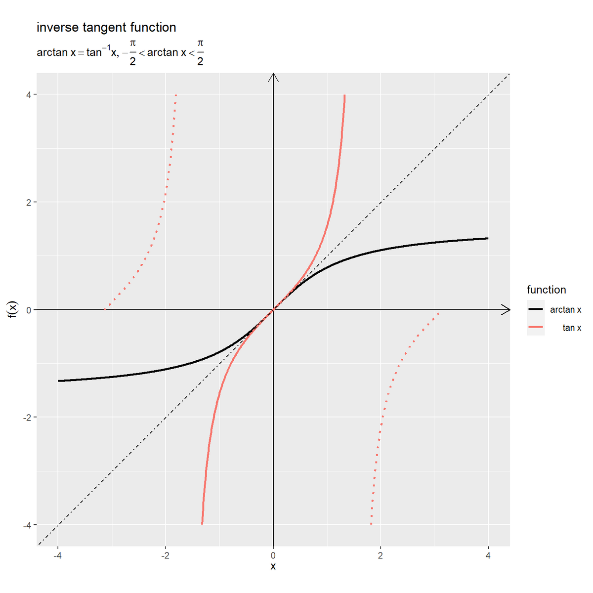
　arctan関数を実線、tan関数を朱色の実線と点線で、また恒等関数 $f(x) = x$ を鎖線で示します。 $\tau = \arctan x$ がとり得る範囲( $-\frac{\pi}{2} \lt \tau \lt \frac{\pi}{2}$ )の $\tan \tau$ を実線で示しています。
　恒等関数(傾きが1で切片が0の直線)に対して、arctan曲線とtan曲線は線対称な曲線です。

　arctan関数の軸を入れ替えたグラフを作成します。

・作図コード(クリックで展開)

tick_num <- 2

# ラジアン軸目盛用の値を作成
rad_break_vec <- seq(from = -pi, to = pi, by = pi/tick_num)
rad_label_vec <- paste(round(rad_break_vec/pi, digits = 2), "* pi")

# 逆関数と元の関数の関係を作図
ggplot() + 
  geom_segment(mapping = aes(x = c(-Inf, 0), y = c(0, -Inf), 
                             xend = c(Inf, 0), yend = c(0, Inf)), 
               arrow = arrow(length = unit(10, units = "pt"), ends = "last")) + # x・y軸線
  geom_vline(xintercept = c(-0.5*pi, 0.5*pi), 
             linetype = "twodash") + # 漸近線
  geom_line(data = curve_inv_df, 
            mapping = aes(x = arctan_x, y = x, color = "arctan"), 
            linewidth = 1) + # 逆関数
  geom_line(data = curve_df,
            mapping = aes(x = t, y = tan_t, color = "tan"), 
            linewidth = 1, linetype = "dashed", na.rm = TRUE) + # 元の関数
  scale_color_manual(breaks = c("arctan", "tan"), 
                     values = c("black", "#F8766D"), 
                     labels = c(expression(arctan~x), expression(tan~theta)), 
                     name = "function") + # 凡例表示用
  scale_x_continuous(breaks = rad_break_vec, 
                     labels = parse(text = rad_label_vec)) + # ラジアン軸目盛
  coord_fixed(ratio = 1) + # アスペクト比
  labs(title = "inverse tangent function", 
       subtitle = parse(text = def_label), 
       x = expression(list(theta, tau == arctan~x)), 
       y = expression(x == tan~theta == tan~tau))

　漸近線を鎖線で示します。
　arctan曲線の横軸と縦軸を入れ替える(恒等関数の直線に対して反転する)と、tan曲線に一致します。

　arctan関数とarccot関数のグラフを作成します。

・作図コード(クリックで展開)

# ラベル用の文字列を作成
def_label <- "arctan~x == frac(pi, 2) - arccot~x"

# 関数曲線を作図
ggplot() + 
  geom_segment(mapping = aes(x = c(-Inf, 0), y = c(0, -Inf), 
                             xend = c(Inf, 0), yend = c(0, Inf)), 
               arrow = arrow(length = unit(10, units = "pt"), ends = "last")) + # x・y軸線
  geom_hline(yintercept = 0.5*pi, 
             linetype = "dashed") + # 余角用の水平線
  geom_line(data = curve_inv_df,
            mapping = aes(x = x, y = arctan_x, linetype = "arctan"), 
            linewidth = 1) + # arctan関数
  geom_line(data = curve_inv_df, 
            mapping = aes(x = x, y = arccot_x, linetype = "arccot"), 
            linewidth = 1) + # arccot関数
  scale_linetype_manual(breaks = c("arctan", "arccot"), 
                        values = c("solid", "dotted"), 
                        labels = c(expression(arctan~x), expression(arccot~x)), 
                        name = "function") + # 凡例表示用
  scale_y_continuous(breaks = rad_break_vec, 
                     labels = parse(text = rad_label_vec)) + # ラジアン軸目盛
  guides(linetype = guide_legend(override.aes = list(linewidth = 0.5))) + # 凡例の体裁
  coord_fixed(ratio = 1, 
              ylim = c(-pi, pi)) + # アスペクト比
  labs(title = "inverse tangent function", 
       subtitle = parse(text = def_label), 
       x = expression(x), 
       y = expression(theta == f(x)))

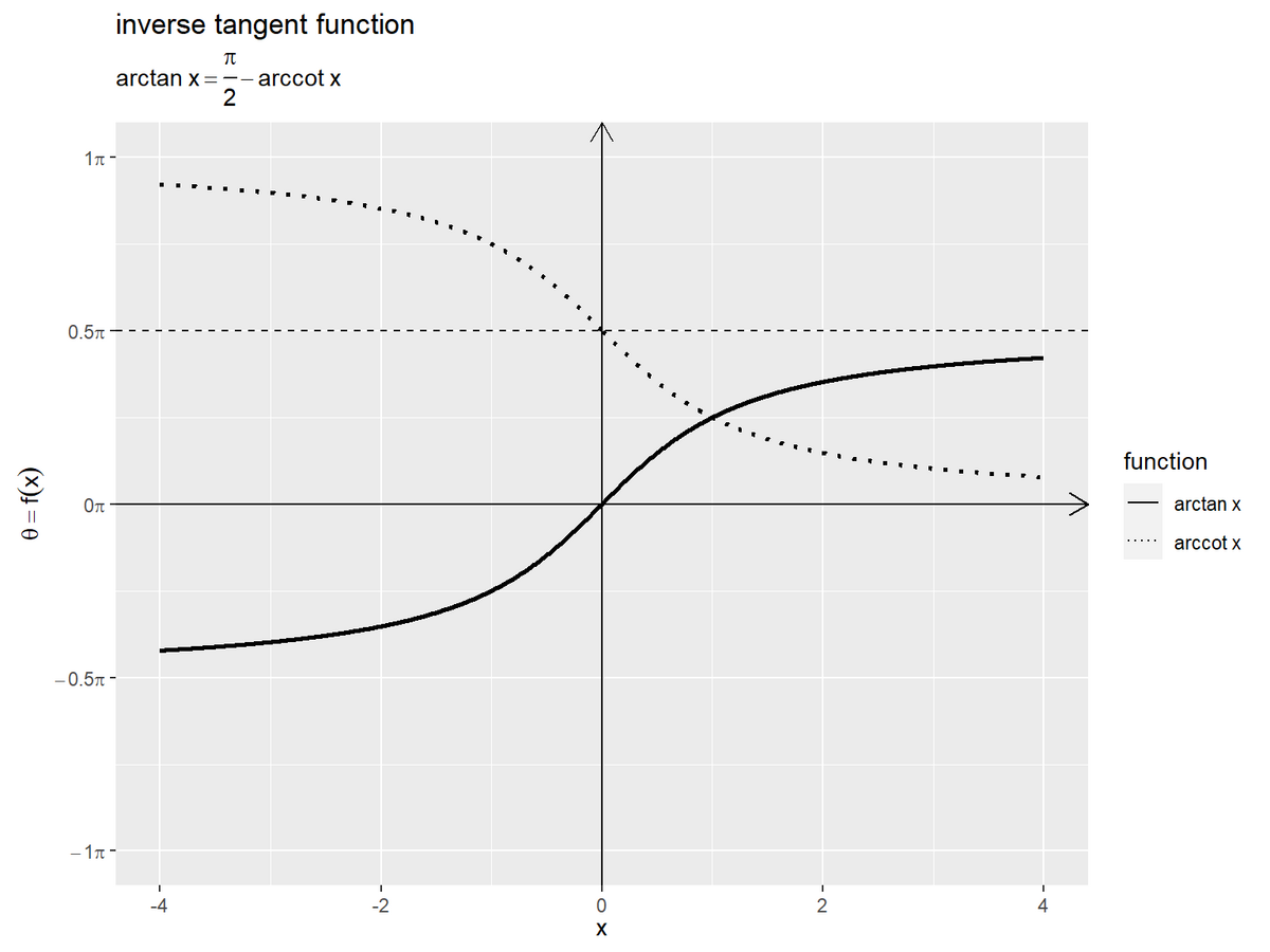
　余角の関係より、 $\arctan x = \frac{\pi}{2} - \mathrm{arccot}\ x$ が成り立ちます。

単位円と関数の関係

　次は、単位円における偏角(単位円上の点)と円関数(tan・sin・cos・exsec)と逆円関数(arctan)の関係を確認します。
　各関数についてはそれぞれの記事を参照してください。

グラフの作成

　変数を固定して、単位円におけるtan関数の線分とarctan関数の円弧のグラフを作成します。

・作図コード(クリックで展開)

　円関数の変数を指定して、逆円関数を計算します。

# 点用のラジアンを指定
theta <- 10/6 * pi

# 終域内のラジアンに変換
tau <- atan(tan(theta))
tau / pi

[1] -0.3333333

　tan関数の変数 $\theta$ を指定して、 $z = \tan \theta$ を変数としてarctan関数 $\tau = \arctan z$ を計算します。

　円周上の点の描画用のデータフレームを作成します。

# 円周上の点の座標を作成
point_df <- tibble::tibble(
  angle = c("theta", "tau"), # 角度カテゴリ
  t = c(theta, tau), 
  x = cos(t), 
  y = sin(t), 
  point_type = c("main", "sub") # 入出力用
)
point_df

# A tibble: 2 × 5
  angle     t     x      y point_type
  <chr> <dbl> <dbl>  <dbl> <chr>     
1 theta  5.24   0.5 -0.866 main      
2 tau   -1.05   0.5 -0.866 sub

　円関数の入力 $\theta$ と逆円関数の出力 $\tau$ それぞれについて、単位円上の点の座標 $(x, y) = (\cos t, \sin t)$ を計算します。

　単位円の描画用のデータフレームを作成します。

# 単位円の座標を作成
circle_df <- tibble::tibble(
  t = seq(from = 0, to = 2*pi, length.out = 361), # 1周期分のラジアン
  r = 1, # 半径
  x = r * cos(t), 
  y = r * sin(t)
)

# 範囲πにおける目盛数を指定
tick_num <- 6

# 角度目盛の座標を作成
rad_tick_df <- tibble::tibble(
  i = seq(from = 0, to = 2*tick_num-0.5, by = 0.5), # 目盛番号
  t = i/tick_num * pi, # ラジアン
  r = 1, # 半径
  x = r * cos(t), 
  y = r * sin(t), 
  major_flag = i%%1 == 0, # 主・補助フラグ
  grid       = dplyr::if_else(major_flag, true = "major", false = "minor") # 目盛カテゴリ
)

　円周と角度軸目盛の座標を作成します。

　偏角の描画用のデータフレームを作成します。

# 半径線の終点の座標を作成
radius_df <- dplyr::bind_rows(
  # 始線
  tibble::tibble(
    x = 1, 
    y = 0, 
    line_type = "main" # 入出力用
  ), 
  # 動径
  point_df |> 
    dplyr::select(x, y, line_type = point_type)
)

# 角マークの座標を作成
d_in  <- 0.2
d_spi <- 0.005
d_out <- 0.3
angle_mark_df <- dplyr::bind_rows(
  # 元の関数の入力
  tibble::tibble(
    angle = "theta", # 角度カテゴリ
    u = seq(from = 0, to = theta, length.out = 600), 
    x = (d_in + d_spi*u) * cos(u), 
    y = (d_in + d_spi*u) * sin(u)
  ), 
  # 逆関数の出力
  tibble::tibble(
    angle = "tau", # 角度カテゴリ
    u = seq(from = 0, to = tau, length.out = 600), 
    x = d_out * cos(u), 
    y = d_out * sin(u)
  )
)

# 角ラベルの座標を作成
d_in  <- 0.1
d_out <- 0.4
angle_label_df <- tibble::tibble(
  u = 0.5 * c(theta, tau), 
  x = c(d_in, d_out) * cos(u), 
  y = c(d_in, d_out) * sin(u), 
  angle_label = c("theta", "tau")
)

　 $\theta, \tau$ それぞれについて、始線と動径、角マークと角ラベルの座標を作成します。

　逆円関数を示す円弧の描画用のデータフレームを作成します。

# 関数円弧の座標を作成
radian_df <- tibble::tibble(
  u = seq(from = 0, to = tau, length.out = 600), 
  r = 1, # 半径
  x = r * cos(u), 
  y = r * sin(u)
)
radian_df

# A tibble: 600 × 4
          u     r     x        y
      <dbl> <dbl> <dbl>    <dbl>
 1  0           1  1     0      
 2 -0.00175     1  1.00 -0.00175
 3 -0.00350     1  1.00 -0.00350
 4 -0.00524     1  1.00 -0.00524
 5 -0.00699     1  1.00 -0.00699
 6 -0.00874     1  1.00 -0.00874
 7 -0.0105      1  1.00 -0.0105 
 8 -0.0122      1  1.00 -0.0122 
 9 -0.0140      1  1.00 -0.0140 
10 -0.0157      1  1.00 -0.0157 
# ℹ 590 more rows

　ラジアン $0 \leq u \leq \tau$ を作成して、単位円の円周上の(半径が $r = 1$ の)円弧の座標 $(x, y) = (\cos u, \sin u)$ を計算します。

　円関数を示す線分の描画用のデータフレームを作成します。

# 関数の描画順を指定
fnc_level_vec <- c("arctan", "tan", "sin", "cos", "exsec")

# 関数線分の座標を作成
fnc_seg_df <- tibble::tibble(
  fnc = c("tan", "sin", "cos", "exsec") |> 
    factor(levels = fnc_level_vec), # 関数カテゴリ
  x_from = c(
    1, 
    cos(theta), 
    0, 
    cos(theta)
  ), 
  y_from = c(
    0, 
    0, 
    0, 
    sin(theta)
  ), 
  x_to = c(
    1, 
    cos(theta), 
    cos(theta), 
    1
  ), 
  y_to = c(
    tan(theta), 
    sin(theta), 
    0, 
    tan(theta)
  )
)
fnc_seg_df

# A tibble: 4 × 5
  fnc   x_from y_from  x_to   y_to
  <fct>  <dbl>  <dbl> <dbl>  <dbl>
1 tan      1    0       1   -1.73 
2 sin      0.5  0       0.5 -0.866
3 cos      0    0       0.5  0    
4 exsec    0.5 -0.866   1   -1.73

　各線分に対応する関数カテゴリを fnc 列として線の描き分けなどに使います。線分の描画順(重なり順や色付け順)を因子レベルで設定します。
　各線分の始点の座標を x_from, y_from 列、終点の座標を x_to, y_to 列として、完成図を見ながら頑張って格納します。

　関数ラベルの描画用のデータフレームを作成します。

# 関数ラベルの座標を作成
fnc_label_df <- tibble::tibble(
  fnc = c("arctan", "tan", "sin", "cos", "exsec") |> 
    factor(levels = fnc_level_vec), # 関数カテゴリ
  x = c(
    cos(0.5 * tau), 
    1, 
    cos(theta), 
    0.5 * cos(theta), 
    0.5 * (cos(theta) + 1)
  ), 
  y = c(
    sin(0.5 * tau),
    0.5 * tan(theta), 
    0.5 * sin(theta), 
    0, 
    0.5 * (sin(theta) + tan(theta))
  ), 
  fnc_label = c("arctan(tan~theta)", "tan~theta", "sin~theta", "cos~theta", "exsec~theta"), 
  a = c( 0,   90,  90,  0,   0), 
  h = c(-0.1, 0.5, 0.5, 0.5, 1.1), 
  v = c( 0.5, 1,  -0.5, 1,   0.5)
)
fnc_label_df

# A tibble: 5 × 7
  fnc        x      y fnc_label             a     h     v
  <fct>  <dbl>  <dbl> <chr>             <dbl> <dbl> <dbl>
1 arctan 0.866 -0.5   arctan(tan~theta)     0  -0.1   0.5
2 tan    1     -0.866 tan~theta            90   0.5   1  
3 sin    0.5   -0.433 sin~theta            90   0.5  -0.5
4 cos    0.25   0     cos~theta             0   0.5   1  
5 exsec  0.75  -1.30  exsec~theta           0   1.1   0.5

　関数ごとに1つの線分の中点に関数名を表示することにします。
　ラベルの表示角度を a 列、表示角度に応じた左右の表示位置を h 列、上下の表示位置を v 列として指定します。

　単位円におけるarctan関数のグラフを作成します。

# ラベル用の文字列を作成
var_label <- paste0(
  "list(", 
  "r == 1, ", 
  "theta == ", round(theta/pi, digits = 2), " * pi, ", 
  "tau == ", round(tau/pi, digits = 2), " * pi", 
  ")"
)
fnc_label_vec <- paste(
  c("arctan(tan~theta)", "tan~theta", "sin~theta", "cos~theta", "exsec~theta"), 
  c(tau, tan(theta), sin(theta), cos(theta), 1/cos(theta)-1) |> 
    round(digits = 2), 
  sep = " == "
)

# グラフサイズの下限値・上限値を指定
axis_lower <- 1.5
axis_upper <- 3

# グラフサイズを設定
axis_x_size <- 1.5
axis_y_min  <- min(-axis_lower, tan(theta)) |> max(-axis_upper)
axis_y_max  <- max(axis_lower, tan(theta)) |> min(axis_upper)

# 単位円における関数線分を作図
ggplot() + 
  geom_segment(data = rad_tick_df, 
               mapping = aes(x = 0, y = 0, xend = x, yend = y, linewidth = grid), 
               color = "white", show.legend = FALSE) + # θ軸目盛線
  geom_segment(mapping = aes(x = c(-Inf, 0), y = c(0, -Inf), 
                             xend = c(Inf, 0), yend = c(0, Inf)),
               arrow = arrow(length = unit(10, units = "pt"), ends = "last")) + # x・y軸線
  geom_path(data = circle_df, 
            mapping = aes(x = x, y = y), 
            linewidth = 1) + # 円周
  geom_segment(data = radius_df, 
               mapping = aes(x = 0, y = 0, xend = x, yend = y, 
                             linewidth = line_type, linetype = line_type), 
               show.legend = FALSE) + # 半径線
  geom_path(data = angle_mark_df, 
            mapping = aes(x = x, y = y, group = angle)) + # 角マーク
  geom_text(data = angle_label_df, 
            mapping = aes(x = x, y = y, label = angle_label), 
            parse = TRUE, size = 5) + # 角ラベル
  geom_text(mapping = aes(x = 0.5*cos(theta+0.1), y = 0.5*sin(theta+0.1)), 
            label = "r", parse = TRUE, 
            size = 5) + # 半径ラベル:(θ + αで表示位置を調整)
  geom_point(data = point_df, 
             mapping = aes(x = x, y = y, shape = point_type), 
             size = 4, show.legend = FALSE) + # 円周上の点
  geom_vline(xintercept = 1, linetype = "dashed") + # 補助線
  geom_path(data = radian_df, 
            mapping = aes(x = x, y = y), 
            color = "red", linewidth = 1) + # 関数円弧
  geom_segment(data = fnc_seg_df, 
               mapping = aes(x = x_from, y = y_from, xend = x_to, yend = y_to, color = fnc), 
               linewidth = 1) + # 関数線分
  geom_text(data = fnc_label_df,
            mapping = aes(x = x, y = y, label = fnc_label, color = fnc,
                          angle = a, hjust = h, vjust = v),
            parse = TRUE, show.legend = FALSE) + # 関数ラベル
  scale_color_manual(breaks = fnc_level_vec, 
                     values = c("red", scales::hue_pal()(n = length(fnc_level_vec)-1)), 
                     labels = parse(text = fnc_label_vec), name = "function") + # 凡例表示用, 色の共通化用
  scale_shape_manual(breaks = c("main", "sub"), 
                     values = c("circle", "circle open")) + # 入出力用
  scale_linetype_manual(breaks = c("main", "sub"), 
                        values = c("solid", "dashed")) + # 入出力用
  scale_linewidth_manual(breaks = c("main", "sub", "major", "minor"), 
                         values = c(1, 0.5, 0.5, 0.25)) + # 入出力用, 主・補助目盛線用
  theme(legend.text.align = 0) + 
  coord_fixed(ratio = 1, 
              xlim = c(-axis_x_size, axis_x_size), 
              ylim = c(axis_y_min, axis_y_max)) + 
  labs(title = "circular functions", 
       subtitle = parse(text = var_label), 
       x = expression(x == r ~ cos~theta), 
       y = expression(y == r ~ sin~theta))

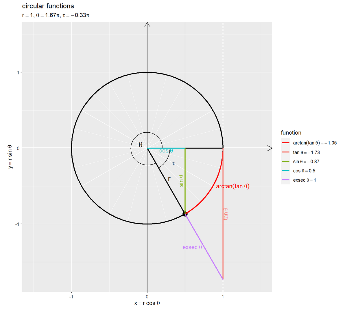
　偏角(x軸の正の部分からの角度)をラジアン $\theta$ とします。中心角が $\theta$ の弧長は $l = r \theta$ です。よって(ラジアンを用いると)、単位円における( $r = 1$ のとき)偏角 $\theta$ と弧長 $l$ が一致します。半径が $r$ の円周上の点の座標は $(x, y) = (r \cos \theta, r \sin \theta)$ です。
　tan関数の値を $z = \tan \theta$ 、arctan関数の値を $\tau = \arctan z$ と置く(tan関数の入力を $\theta$ 、arctan関数の出力を $\tau$ とする)と、tan関数が $z$ になる偏角(弧長)が $\tau$ であり、 $\tan \theta = \tan \tau$ となります。

アニメーションの作成

　変数を変化させて、単位円におけるarctan関数のアニメーションを作成します。
　作図コードについては「GitHub - anemptyarchive/Mathematics/.../arctan_definition.R」を参照してください。

　単位円における偏角とarctan関数の円弧の関係を可視化します。

　tan関数の終域 $-\infty \leq \tan \theta \leq \infty$ をarctan関数の定義域 $-\infty \leq z \leq \infty$ として、終域が $-\frac{\pi}{2} \leq \arctan z \leq \frac{\pi}{2}$ になるのを確認できます。