はじめに
そろそろ真面目に三角関数の勉強を始めましょうかシリーズ(仮)です。
この記事では、R言語でサイン波の変形を可視化します。
【前の内容】
【この記事の内容】
sin関数の振幅・周期・平行移動の変形の可視化
sin関数に関して、関数または変数の係数や定数項による波の振幅・周期・平行移動の変化をグラフで確認します。sin関数の作図については「【R】sin関数の可視化 - からっぽのしょこ」を参照してください。
利用するパッケージを読み込みます。
# 利用パッケージ
library(tidyverse)
library(patchwork)
library(magick)
この記事では、基本的にパッケージ名::関数名()の記法を使うので、パッケージを読み込む必要はありません。ただし、作図コードがごちゃごちゃしないようにパッケージ名を省略しているためggplot2を読み込む必要があります。
また、ネイティブパイプ演算子|>を使っています。magrittrパッケージのパイプ演算子%>%に置き換えても処理できますが、その場合はmagrittrも読み込む必要があります。
関数をk倍する場合
まずは、sin関数$\sin \theta$の係数と振幅の関係を可視化します。
グラフの作成
角度$\theta$を固定した$k \sin \theta$をグラフで確認します。
関数の係数と角度を指定します。
# 関数の係数を指定
k <- 3

# 角度を指定
alpha <- 120

# ラジアンに変換
theta <- alpha / 180 * pi
theta
## [1] 2.094395
sin関数の係数$k$を指定します。
度数法における角度$\alpha$を指定して、弧度法における角度(ラジアン)$\theta = \alpha \frac{\pi}{180}$に変換します。$\pi$は円周率でpiで扱えます。
・コード(クリックで展開)
曲線上に関数の点を描画するためのデータフレームを作成します。
# 関数の点の描画用
point_df <- tibble::tibble(
  theta = theta,
  sin_theta = sin(theta) * c(1, k),
  cos_theta = cos(theta) * c(1, k),
  fnc = c("sin theta", "k sin theta")
)
point_df
## # A tibble: 2 × 4
##   theta sin_theta cos_theta fnc
##   <dbl>     <dbl>     <dbl> <chr>
## 1  2.09     0.866      -0.5 sin theta
## 2  2.09     2.60       -1.5 k sin theta
sin関数$\sin \theta$とk倍したsin関数$k \sin \theta$、cos関数$\cos \theta$とk倍したcos関数$k \cos \theta$を計算して、$\theta$と共に格納します。(オブジェクト名と列名が重複するため、エラーにならないように処理しています。)
作図時の色分けなど用に、元の関数とk倍した値を区別するための列fncを作成します。
単位円とk倍した円を描画するためのデータフレームを作成します。
# 単位円の描画用
tmp_vals <- seq(from = 0, to = 2*pi, by = 0.05)
circle_df <- tibble::tibble(
  theta = c(tmp_vals, tmp_vals),
  sin_theta = c(sin(tmp_vals), sin(tmp_vals)*k),
  cos_theta = c(cos(tmp_vals), cos(tmp_vals)*k),
  fnc = rep(c("sin theta", "k sin theta"), each = length(tmp_vals))
)
circle_df
## # A tibble: 252 × 4
##    theta sin_theta cos_theta fnc
##    <dbl>     <dbl>     <dbl> <chr>
##  1  0       0          1     sin theta
##  2  0.05    0.0500     0.999 sin theta
##  3  0.1     0.0998     0.995 sin theta
##  4  0.15    0.149      0.989 sin theta
##  5  0.2     0.199      0.980 sin theta
##  6  0.25    0.247      0.969 sin theta
##  7  0.3     0.296      0.955 sin theta
##  8  0.35    0.343      0.939 sin theta
##  9  0.4     0.389      0.921 sin theta
## 10  0.45    0.435      0.900 sin theta
## # … with 242 more rows
単位円の作図用のラジアン$0 \leq \theta \leq 2 \pi$を作成して、$\sin \theta, \cos \theta$を計算します。単位円の座標は、x軸の値$x = \cos \theta$、y軸の値$y = \sin \theta$に対応します。
同様に、k倍した値も格納します。こちらは、半径が$k$の円周上の点になります。
単位円上に角度目盛を描画するためのデータフレームを作成します。
# 角度目盛の描画用
tick_df <- tibble::tibble(
  alpha = 0:11 * 30,
  theta = 0:11 / 6 * pi,
  x = cos(theta),
  y = sin(theta),
  rad_label = paste0("frac(", 0:11, ", 6)~pi")
)
tick_df
## # A tibble: 12 × 5
##    alpha theta         x         y rad_label
##    <dbl> <dbl>     <dbl>     <dbl> <chr>
##  1     0 0      1   e+ 0  0        frac(0, 6)~pi
##  2    30 0.524  8.66e- 1  5   e- 1 frac(1, 6)~pi
##  3    60 1.05   5   e- 1  8.66e- 1 frac(2, 6)~pi
##  4    90 1.57   6.12e-17  1   e+ 0 frac(3, 6)~pi
##  5   120 2.09  -5   e- 1  8.66e- 1 frac(4, 6)~pi
##  6   150 2.62  -8.66e- 1  5   e- 1 frac(5, 6)~pi
##  7   180 3.14  -1   e+ 0  1.22e-16 frac(6, 6)~pi
##  8   210 3.67  -8.66e- 1 -5   e- 1 frac(7, 6)~pi
##  9   240 4.19  -5.00e- 1 -8.66e- 1 frac(8, 6)~pi
## 10   270 4.71  -1.84e-16 -1   e+ 0 frac(9, 6)~pi
## 11   300 5.24   5   e- 1 -8.66e- 1 frac(10, 6)~pi
## 12   330 5.76   8.66e- 1 -5.00e- 1 frac(11, 6)~pi
$30^{\circ} = 30 \frac{\pi}{180} = \frac{\pi}{6}$間隔で、$\frac{n}{6} \pi\ (n = 0, \dots, 11)$の形で目盛を表示することにします。
単位円のときと同様に、x軸とy軸の値を計算して、ラベルと合わせて格納します。ラベルとして数式を表示する場合は、expression()の記法を使います。
角度を表示するためのデータフレームを作成します。
# 半径の描画用
radius_df <- tibble::tibble(
  x_from = c(0, 0, 0),
  y_from = c(0, 0, 0),
  x_to = c(1, cos(theta), cos(theta)*k),
  y_to = c(0, sin(theta), sin(theta)*k),
  fnc = c("r", "sin theta", "k sin theta")
)

# 角度マークの描画用
d <- 0.1
angle_df <- tibble::tibble(
  theta = seq(from = min(0, theta), to = max(0, theta), length.out = 100),
  x = cos(theta) * d,
  y = sin(theta) * d
)

# 角度ラベルの描画用
d <- 0.2
angle_label_df <- tibble::tibble(
  theta = 0.5 * theta,
  x = cos(theta) * d,
  y = sin(theta) * d,
  angle_label = "theta"
)
radius_df; angle_df; angle_label_df
## # A tibble: 3 × 5
##   x_from y_from  x_to  y_to fnc
##    <dbl>  <dbl> <dbl> <dbl> <chr>
## 1      0      0   1   0     r
## 2      0      0  -0.5 0.866 sin theta
## 3      0      0  -1.5 2.60  k sin theta
## # A tibble: 100 × 3
##     theta      x       y
##     <dbl>  <dbl>   <dbl>
##  1 0      0.1    0
##  2 0.0212 0.100  0.00212
##  3 0.0423 0.0999 0.00423
##  4 0.0635 0.0998 0.00634
##  5 0.0846 0.0996 0.00845
##  6 0.106  0.0994 0.0106
##  7 0.127  0.0992 0.0127
##  8 0.148  0.0989 0.0148
##  9 0.169  0.0986 0.0168
## 10 0.190  0.0982 0.0189
## # … with 90 more rows
## # A tibble: 1 × 4
##   theta     x     y angle_label
##   <dbl> <dbl> <dbl> <chr>
## 1  1.05   0.1 0.173 theta
$0^{\circ}, \theta$のそれぞれの角度における半径を描画するために、原点と円周上の点を結ぶ線分の座標を格納してradius_dfとします。始点の座標をx_from, y_from、終点の座標をx_to, y_to列とします。
扇形(角度マーク)を描画するための値(ラジアン)を作成して、x軸とy軸の値を計算してangle_dfとします。$\theta$が正の値($\theta > 0$)のときは$0$から$\theta$、負の値($\theta < 0$)のときは$\theta$から$0$の値となるように処理します。
角度の中点に配置するように座標とラベル用の文字列を格納してangle_label_dfとします。
単位円におけるsin関数の値を描画するためのデータフレームを作成します。
# sin関数の線の描画用
sin_line_df <- tibble::tibble(
  x_from = c(cos(theta), cos(theta)*k),
  y_from = c(0, 0),
  x_to = c(cos(theta), cos(theta)*k),
  y_to = c(sin(theta), sin(theta)*k),
  fnc = c("sin theta", "k sin theta")
)

# sin関数の線ラベルの描画用
sin_label_df <- sin_line_df |>
  dplyr::group_by(fnc) |> # 中点の計算用
  dplyr::mutate(
    # 中点に配置
    x = median(c(x_from, x_to)),
    y = median(c(y_from, y_to))
  ) |>
  dplyr::ungroup() |>
  tibble::add_column(
    fnc_label = c("sin~theta", "k~sin~theta")
  ) |>
  dplyr::select(x, y, fnc, fnc_label)
sin_line_df; sin_label_df
## # A tibble: 2 × 5
##   x_from y_from  x_to  y_to fnc
##    <dbl>  <dbl> <dbl> <dbl> <chr>
## 1   -0.5      0  -0.5 0.866 sin theta
## 2   -1.5      0  -1.5 2.60  k sin theta
## # A tibble: 2 × 4
##       x     y fnc         fnc_label
##   <dbl> <dbl> <chr>       <chr>
## 1  -0.5 0.433 sin theta   sin~theta
## 2  -1.5 1.30  k sin theta k~sin~theta
sin関数の値は、角度$\theta$における単位円上の点$(\cos \theta, \sin \theta)$と、$x = 0$の直線への垂線との交点$(\cos \theta, 0)$を結ぶ線分で表現できます。同様に、k倍した値も格納します。それぞれ始点と終点の座標を格納してsin_line_dfとします。
sin関数の垂線(線分)の中点に配置するように座標とラベル用の文字列を格納してsin_label_dfとします。
単位円上の点とsin関数上の点を結ぶ線(の半分)を描画するためのデータフレームを作成します。
# 描画領域のサイズを設定
axis_size <- max(1, abs(k)) + 0.5
l         <- 1.5

# サイン波との対応用
segment_circle_df <- tibble::tibble(
  x_from = c(cos(theta), cos(theta)*k),
  y_from = c(sin(theta), sin(theta)*k),
  x_to = c(-axis_size-l, -axis_size-l),
  y_to = c(sin(theta), sin(theta)*k),
  fnc = c("sin theta", "k sin theta")
)
segment_circle_df
## # A tibble: 2 × 5
##   x_from y_from  x_to  y_to fnc
##    <dbl>  <dbl> <dbl> <dbl> <chr>
## 1   -0.5  0.866    -5 0.866 sin theta
## 2   -1.5  2.60     -5 2.60  k sin theta
円周上の点からy軸への垂線を引くように座標を指定します。作図時に、隣のグラフに届かないような長さlを指定します。
また、2つのグラフの描画範囲を固定するために、axis_sizeとして値を指定しておきます。
単位円のグラフを作成します。
# 関数ラベルを作成
fnc_label <- paste0(
  "list(",
  "theta==", round(theta/pi, digits = 2), "*pi",
  ", k==", k,
  ", sin~theta==", round(sin(theta), digits = 2),
  ", cos~theta==", round(cos(theta), digits = 2),
  ")"
)

# 単位円を作図
d <- 1.2
circle_graph <- ggplot() +
  geom_path(data = circle_df,
            mapping = aes(x = cos_theta, y = sin_theta, group = fnc, linetype = fnc),
            size = 1) + # 単位円
  geom_text(data = tick_df,
            mapping = aes(x = x, y = y, angle = alpha+90),
            label = "|", size = 2) + # 角度目盛
  geom_text(data = tick_df,
            mapping = aes(x = x*d, y = y*d, label = rad_label,
                          hjust = 1-(x*0.5+0.5), vjust = 1-(y*0.5+0.5)), parse = TRUE) + # 角度目盛ラベル
  geom_segment(data = radius_df,
               mapping = aes(x = x_from, y = y_from, xend = x_to, yend = y_to, linetype = fnc)) + # 半径
  geom_path(data = angle_df,
            mapping = aes(x = x, y = y)) + # 角度マーク
  geom_text(data = angle_label_df,
            mapping = aes(x = x, y = y, label = angle_label), parse = TRUE) + # 角度ラベル
  geom_segment(data = sin_line_df,
               mapping = aes(x = x_from, y = y_from, xend = x_to, yend = y_to, color = fnc),
               size = 1) + # sin関数
  geom_text(data = sin_label_df,
             mapping = aes(x = x, y = y, label = fnc_label, color = fnc), parse = TRUE,
             angle = 90, vjust = 1) + # sin関数ラベル
  geom_segment(data = segment_circle_df,
               mapping = aes(x = x_from, y = y_from, xend = x_to, yend = y_to),
               linetype = "dotted") + # sin波との対応線
  geom_point(data = point_df,
             mapping = aes(x = cos_theta, y = sin_theta),
             size = 4) + # 円上の点
  scale_color_manual(breaks = c("sin theta", "k sin theta"),
                     values = c("red", "blue")) + # 線の色
  scale_linetype_manual(breaks = c("sin theta", "k sin theta", "r"),
                        values = c("solid", "dashed", "solid")) + # 線の種類
  theme(legend.position = "none") + # 凡例の非表示
  coord_fixed(ratio = 1, clip = "off",
              xlim = c(-axis_size, axis_size), ylim = c(-axis_size, axis_size)) + # 描画領域
  labs(title = "unit circle",
       subtitle = parse(text = fnc_label),
       x = "x", y = "y")
circle_graph

x軸をcos関数の値、y軸をsin関数の値として、(geom_line()ではなく)geom_path()で曲線(円)を描画します。綺麗な円を描画するにはcoord_***()のratio引数を1にします。
ラベル配置位置の調整用の値をdとして、tick_dfを使って角度ラベルを描画します。また、x軸・y軸方向の配置位置の調整用の引数hjust, yjustに、x, y列の値を使って指定しています。x, y列($\sin \theta, \cos \theta$)は―1から1の値をとります。0.5を掛けると-0.5から0.5の値となり、さらに0.5を足すと0から1の値になります。(hjust, vjustを指定せずにdを少し大きくしても同様の図になります。)
半径などの線分をgeom_segment()で描画します。
サイン波の作図用のラジアンの値を作成します。
# 作図用のラジアンの値を作成
theta_vals <- seq(from = theta-2*pi, to = theta+2*pi, by = 0.01)
head(theta_vals)
## [1] -4.18879 -4.17879 -4.16879 -4.15879 -4.14879 -4.13879
この例では、指定した$\theta$を中心に前後$2 \pi$を範囲とします。範囲(サイズ)を$2 \pi$にすると、1周期分の曲線を描画できます。この例は、2周期になります。
サイン波の描画するためのデータフレームを作成します。
# サイン波の描画用
sin_curve_df <- tibble::tibble(
  theta = c(theta_vals, theta_vals),
  sin_theta = c(sin(theta_vals), sin(theta_vals)*k),
  fnc = rep(c("sin theta", "k sin theta"), each = length(theta_vals))
)
sin_curve_df
## # A tibble: 2,514 × 3
##    theta sin_theta fnc
##    <dbl>     <dbl> <chr>
##  1 -4.19     0.866 sin theta
##  2 -4.18     0.861 sin theta
##  3 -4.17     0.856 sin theta
##  4 -4.16     0.851 sin theta
##  5 -4.15     0.845 sin theta
##  6 -4.14     0.840 sin theta
##  7 -4.13     0.834 sin theta
##  8 -4.12     0.829 sin theta
##  9 -4.11     0.823 sin theta
## 10 -4.10     0.818 sin theta
## # … with 2,504 more rows
作図用の$\theta$の値と$\sin \theta, k \sin \theta$の値を格納します。
先ほどと同様に、sin関数上の点と円周上の点を結ぶ線(の半分)を描画するためのデータフレームを作成します。
# x軸(角度)・単位円との対応用
d <- 1.1
segment_sin_df <- tibble::tibble(
  x_from = c(theta, theta, theta, theta),
  y_from = c(sin(theta), sin(theta), sin(theta)*k, sin(theta)*k),
  x_to = c(theta, max(theta_vals)+l, theta, max(theta_vals)+l),
  y_to = c(-axis_size*d, sin(theta), -axis_size*d, sin(theta)*k),
  fnc = rep(c("sin theta", "k sin theta"), each = 2)
)
segment_sin_df
## # A tibble: 4 × 5
##   x_from y_from  x_to   y_to fnc
##    <dbl>  <dbl> <dbl>  <dbl> <chr>
## 1   2.09  0.866  2.09 -3.85  sin theta
## 2   2.09  0.866  9.87  0.866 sin theta
## 3   2.09  2.60   2.09 -3.85  k sin theta
## 4   2.09  2.60   9.87  2.60  k sin theta
曲線上の点からx軸・y軸への垂線を引くように座標を指定します。
x軸目盛として、角度ラベルを描画するのに用いるベクトルを作成します。
# x軸目盛ラベルの描画用の値を作成
tick_min <- floor(min(theta_vals) * 6 / pi)
tick_vec <- seq(from = tick_min, to = tick_min+25, by = 1)
tick_vec
##  [1] -9 -8 -7 -6 -5 -4 -3 -2 -1  0  1  2  3  4  5  6  7  8  9 10 11 12 13 14 15
## [26] 16
単位円の目盛と同様に、$30^{\circ} = \frac{\pi}{6}$間隔で目盛を表示することにします。$\frac{n}{6} \pi$の形で目盛を描画するために、作図用の角度$\theta$の最小値を、floor()で小数点以下を切り捨てて、$\frac{6}{\pi}$倍して、最小値の$n$を求めてtick_minとします。
theta_valsのサイズが$4 \pi$の場合は、$n$から$n+25$までの整数を生成してtick_vecとします。
サイン波のグラフを作成します。
# 関数ラベルを作成
fnc_label <- paste0(
  "list(",
  "theta==", round(theta/pi, digits = 2), "*pi",
  ", k==", k,
  ", sin~theta==", round(sin(theta), digits = 2),
  ", k~sin~theta==", round(sin(theta)*k, digits = 2),
  ")"
)

# サイン波を作図
sin_graph <- ggplot() +
  geom_line(data = sin_curve_df,
            mapping = aes(x = theta, y = sin_theta, color = fnc),
            size = 1) + # sin関数
  geom_segment(data = segment_sin_df,
               mapping = aes(x = x_from, y = y_from, xend = x_to, yend = y_to),
               linetype = "dotted") + # 単位円との対応線
  geom_point(data = point_df,
             mapping = aes(x = theta, y = sin_theta),
             size = 4) + # 関数曲線上の点
  scale_x_continuous(breaks = tick_vec/6*pi,
                     labels = parse(text = paste0("frac(", tick_vec, ", 6)~pi"))) + # 角度目盛ラベル
  scale_color_manual(breaks = c("sin theta", "k sin theta"),
                     values = c("red", "blue"),
                     labels = parse(text = c("sin~theta", "k~sin~theta")),
                     name = "function") + # 線の色
  coord_fixed(ratio = 1, clip = "off",
              xlim = c(min(theta_vals), max(theta_vals)), ylim = c(-axis_size, axis_size)) + # 描画領域
  labs(title = "sine curve",
       subtitle = parse(text = fnc_label),
       x = expression(theta), y = expression(f(theta)))
sin_graph
x軸を$\theta$、y軸をsin関数の値としてgeom_line()で曲線を描画します。
scale_x_continuous()でx軸目盛を設定します。目盛の表示位置の引数breaksにtick_vecを$\frac{\pi}{6}$倍した値、目盛ラベルの引数labelsに$\frac{n}{6} \pi$の形の文字列を指定します。
2つのグラフを並べて描画します。
# グラフを並べて描画
patchwork::wrap_plots(sin_graph, circle_graph) +
  patchwork::plot_layout(guides = "collect")
patchworkパッケージのwrap_plots()を使ってグラフを並べます。
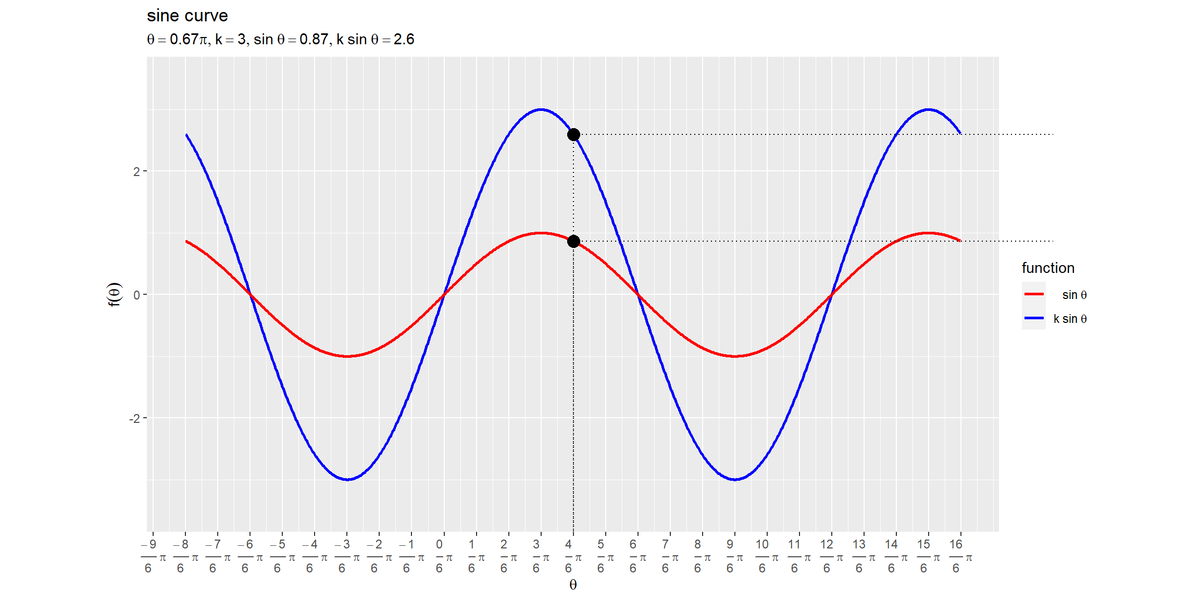
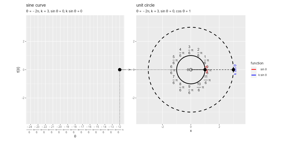
・$\theta^{\circ} = 120^{\circ}, k = 3$のグラフ
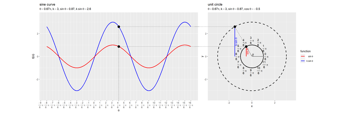
点$(k \cos \theta, k \sin \theta)$は、半径がkの円(単位円をk倍した円)上の点になります。よって、サイン波の振幅もk倍になるのを確認できます。
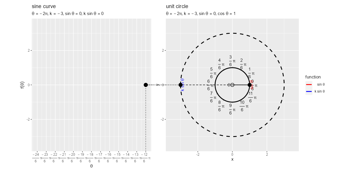
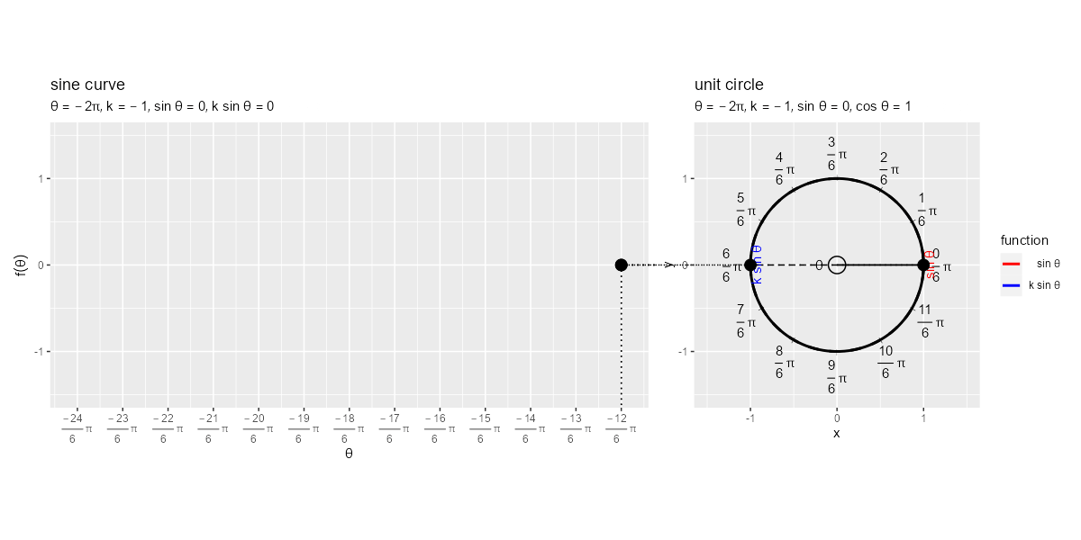
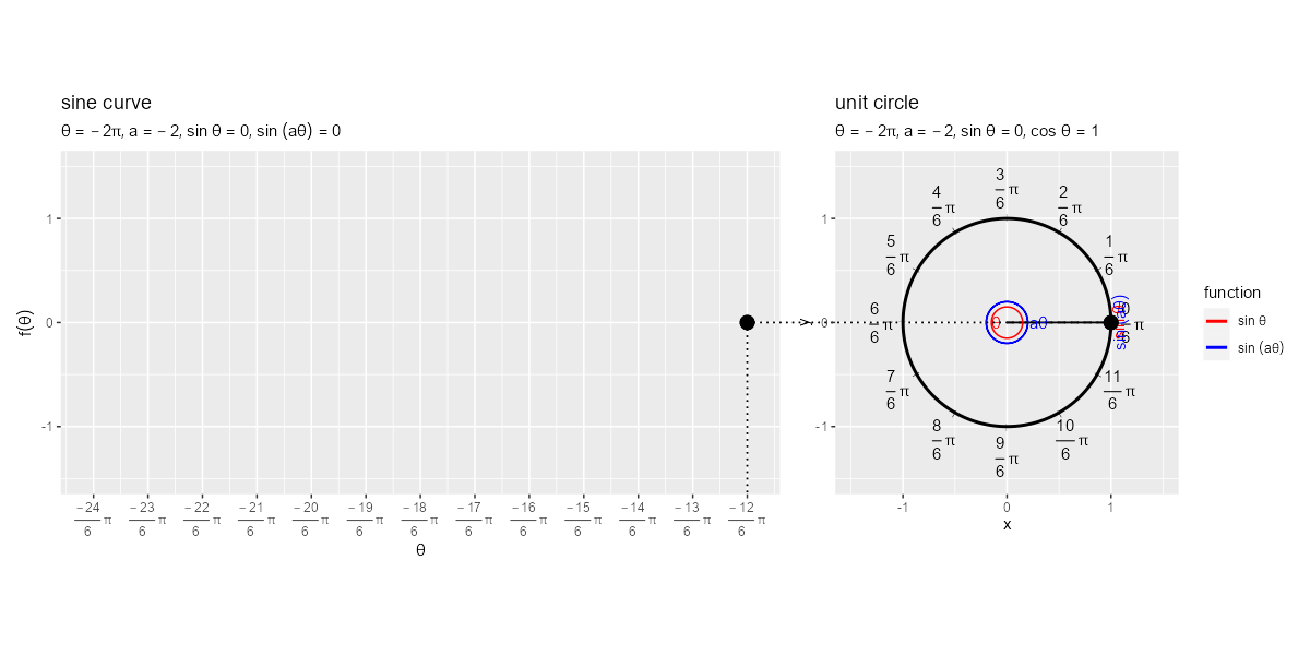
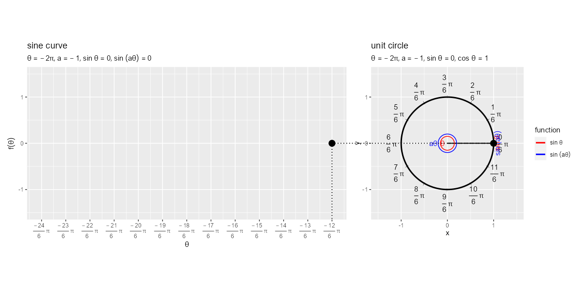
・$\theta^{\circ} = 120^{\circ}, k = -1$のグラフ
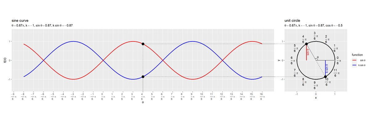
$k$が負の値のとき、円周上の点については原点に対して反転し、サイン波については$x = 0$の直線に対して反転したグラフになります。また、「変数をa倍する場合」で確認する$a = -1$のとき、「変数にbを加える場合」で確認する$b = \pi = 180^{\circ}$のときと同じグラフになることから、$-\sin \theta = \sin(-\theta) = \sin(\theta + 180^{\circ})$が成り立つのを確認できます。
・$\theta^{\circ} = 120^{\circ}, k = \frac{1}{2}$のグラフ
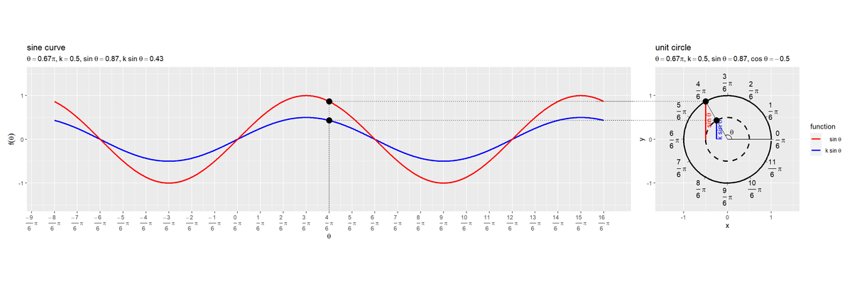
$k$が1未満のときは、単位円(振幅が-1から1)よりも小さくなります。
アニメーションの作成
続いて、角度を変化させたアニメーションで確認します。
フレーム数と角度の範囲を指定して、角度として用いる値を作成します。
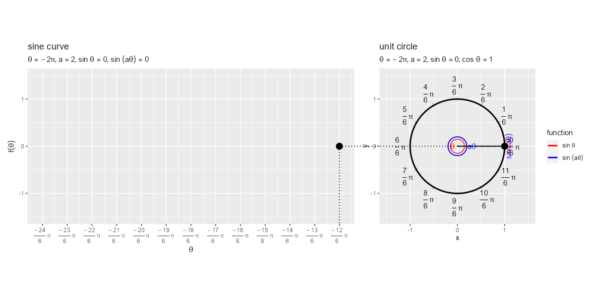
# フレーム数を指定
frame_num <- 100

# 関数の係数を指定
k <- 3

# 角度の範囲を指定
theta_min <- -2 * pi
theta_max <- 2 * pi

# フレームごとの角度を作成
theta_i <- seq(from = theta_min, to = theta_max, length.out = frame_num+1)[1:frame_num]
head(theta_i)
## [1] -6.283185 -6.157522 -6.031858 -5.906194 -5.780530 -5.654867
フレーム数frame_numと、角度(ラジアン)$\theta$の最小値theta_min・最大値theta_maxを指定して、frame_num個の等間隔の$\theta$の値を作成します。三角関数は$2 \pi$で1周期なので、最小値に$2 \pi$の$n$倍を加えた値を最大値にして、等間隔に切り分け最大値自体を除くと、最後のフレームと最初のフレームの繋がりが良くなります。
・コード(クリックで展開)
theta_iから順番に値を取り出して作図し、グラフを書き出します
# 一時保存フォルダを指定
dir_path <- "tmp_folder"

# 描画領域のサイズを設定
axis_size <- max(1, abs(k)) + 0.5
l         <- 1.5

# 単位円の描画用
tmp_vals <- seq(from = 0, to = 2*pi, by = 0.05)
circle_df <- tibble::tibble(
  theta = c(tmp_vals, tmp_vals),
  sin_theta = c(sin(tmp_vals), sin(tmp_vals)*k),
  cos_theta = c(cos(tmp_vals), cos(tmp_vals)*k),
  fnc = rep(c("sin theta", "k sin theta"), each = length(tmp_vals))
)

# 角度ごとに作図
for(i in 1:frame_num) {

  # i番目の角度を取得
  theta <- theta_i[i]

  # 関数の点の描画用
  point_df <- tibble::tibble(
    theta = theta,
    sin_theta = sin(theta) * c(1, k),
    cos_theta = cos(theta) * c(1, k),
    fnc = c("sin theta", "k sin theta")
  )

  # 半径の描画用
  radius_df <- tibble::tibble(
    x_from = c(0, 0, 0),
    y_from = c(0, 0, 0),
    x_to = c(1, cos(theta), cos(theta)*k),
    y_to = c(0, sin(theta), sin(theta)*k),
    fnc = c("r", "sin theta", "k sin theta")
  )

  # 角度マークの描画用
  d <- 0.1
  angle_df <- tibble::tibble(
    theta = seq(from = min(0, theta), to = max(0, theta), length.out = 100),
    x = cos(theta) * d,
    y = sin(theta) * d
  )

  # 角度ラベルの描画用
  d <- 0.2
  angle_label_df <- tibble::tibble(
    theta = 0.5 * theta,
    x = cos(theta) * d,
    y = sin(theta) * d,
    angle_label = "theta"
  )

  # sin関数の線の描画用
  sin_line_df <- tibble::tibble(
    x_from = c(cos(theta), cos(theta)*k),
    y_from = c(0, 0),
    x_to = c(cos(theta), cos(theta)*k),
    y_to = c(sin(theta), sin(theta)*k),
    fnc = c("sin theta", "k sin theta")
  )

  # sin関数の線ラベルの描画用
  sin_label_df <- sin_line_df |>
    dplyr::group_by(fnc) |> # 中点の計算用
    dplyr::mutate(
      # 中点に配置
      x = median(c(x_from, x_to)),
      y = median(c(y_from, y_to))
    ) |>
    dplyr::ungroup() |>
    tibble::add_column(
      fnc_label = c("sin~theta", "k~sin~theta")
    ) |>
    dplyr::select(x, y, fnc, fnc_label)

  # サイン波との対応用
  segment_circle_df <- tibble::tibble(
    x_from = c(cos(theta), cos(theta)*k),
    y_from = c(sin(theta), sin(theta)*k),
    x_to = c(-axis_size-l, -axis_size-l),
    y_to = c(sin(theta), sin(theta)*k),
    fnc = c("sin theta", "k sin theta")
  )

  # 関数ラベルを作成
  fnc_label <- paste0(
    "list(",
    "theta==", round(theta/pi, digits = 2), "*pi",
    ", k==", k,
    ", sin~theta==", round(sin(theta), digits = 2),
    ", cos~theta==", round(cos(theta), digits = 2),
    ")"
  )

  # 単位円を作図
  d <- 1.2
  circle_graph <- ggplot() +
    geom_path(data = circle_df,
              mapping = aes(x = cos_theta, y = sin_theta, group = fnc, linetype = fnc),
              size = 1) + # 単位円
    geom_text(data = tick_df,
              mapping = aes(x = x, y = y, angle = alpha+90),
              label = "|", size = 2) + # 角度目盛
    geom_text(data = tick_df,
              mapping = aes(x = x*d, y = y*d, label = rad_label,
                            hjust = 1-(x*0.5+0.5), vjust = 1-(y*0.5+0.5)), parse = TRUE) + # 角度目盛ラベル
    geom_segment(data = radius_df,
                 mapping = aes(x = x_from, y = y_from, xend = x_to, yend = y_to, linetype = fnc)) + # 半径
    geom_path(data = angle_df,
              mapping = aes(x = x, y = y)) + # 角度マーク
    geom_text(data = angle_label_df,
              mapping = aes(x = x, y = y, label = angle_label), parse = TRUE) + # 角度ラベル
    geom_segment(data = sin_line_df,
                 mapping = aes(x = x_from, y = y_from, xend = x_to, yend = y_to, color = fnc),
                 size = 1) + # sin関数
    geom_text(data = sin_label_df,
               mapping = aes(x = x, y = y, label = fnc_label, color = fnc), parse = TRUE,
               angle = 90, vjust = 1) + # sin関数ラベル
    geom_segment(data = segment_circle_df,
                 mapping = aes(x = x_from, y = y_from, xend = x_to, yend = y_to),
                 linetype = "dotted") + # sin波との対応線
    geom_point(data = point_df,
               mapping = aes(x = cos_theta, y = sin_theta),
               size = 4) + # 円上の点
    scale_color_manual(breaks = c("sin theta", "k sin theta"),
                       values = c("red", "blue")) + # 線の色
    scale_linetype_manual(breaks = c("sin theta", "k sin theta", "r"),
                          values = c("solid", "dashed", "solid")) + # 線の種類
    theme(legend.position = "none") + # 凡例の非表示
    coord_fixed(ratio = 1, clip = "off",
                xlim = c(-axis_size, axis_size), ylim = c(-axis_size, axis_size)) + # 描画領域
    labs(title = "unit circle",
         subtitle = parse(text = fnc_label),
         x = "x", y = "y")

  # 作図用のラジアンの値を作成
  theta_size <- 2 * pi
  theta_vals <- seq(from = max(theta_min, theta-theta_size), to = theta, by = 0.01)

  # サイン波の描画用
  sin_curve_df <- tibble::tibble(
    theta = c(theta_vals, theta_vals),
    sin_theta = c(sin(theta_vals), sin(theta_vals)*k),
    fnc = rep(c("sin theta", "k sin theta"), each = length(theta_vals))
  )

  # x軸(角度)・単位円との対応用
  d <- 1.1
  segment_sin_df <- tibble::tibble(
    x_from = c(theta, theta, theta, theta),
    y_from = c(sin(theta), sin(theta), sin(theta)*k, sin(theta)*k),
    x_to = c(theta, max(theta_vals)+l, theta, max(theta_vals)+l),
    y_to = c(-axis_size*d, sin(theta), -axis_size*d, sin(theta)*k),
    fnc = rep(c("sin theta", "k sin theta"), each = 2)
  )

  # x軸目盛ラベルの描画用の値を作成
  tick_min <- floor((theta-theta_size) * 6 / pi)
  tick_vec <- seq(from = tick_min, to = tick_min+13, by = 1)

  # 関数ラベルを作成
  fnc_label <- paste0(
    "list(",
    "theta==", round(theta/pi, digits = 2), "*pi",
    ", k==", k,
    ", sin~theta==", round(sin(theta), digits = 2),
    ", k~sin~theta==", round(sin(theta)*k, digits = 2),
    ")"
  )

  # サイン波を作図
  sin_graph <- ggplot() +
    geom_line(data = sin_curve_df,
              mapping = aes(x = theta, y = sin_theta, color = fnc),
              size = 1) + # sin関数
    geom_segment(data = segment_sin_df,
                 mapping = aes(x = x_from, y = y_from, xend = x_to, yend = y_to),
                 linetype = "dotted") + # 単位円との対応線
    geom_point(data = point_df,
               mapping = aes(x = theta, y = sin_theta),
               size = 4) + # 関数曲線上の点
    scale_x_continuous(breaks = tick_vec/6*pi,
                       labels = parse(text = paste0("frac(", tick_vec, ", 6)~pi"))) + # 角度目盛ラベル
    scale_color_manual(breaks = c("sin theta", "k sin theta"),
                       values = c("red", "blue"),
                       labels = parse(text = c("sin~theta", "k~sin~theta")),
                       name = "function") + # 線の色
    #theme(legend.position = "none") + # 凡例の非表示
    coord_fixed(ratio = 1, clip = "off",
                xlim = c(theta-theta_size, theta), ylim = c(-axis_size, axis_size)) + # 描画領域
    labs(title = "sine curve",
         subtitle = parse(text = fnc_label),
         x = expression(theta), y = expression(f(theta)))

  # グラフを並べて描画
  graph <- patchwork::wrap_plots(sin_graph, circle_graph) +
      patchwork::plot_layout(guides = "collect")

  # ファイルを書き出し
  file_path <- paste0(dir_path, "/", stringr::str_pad(i, width = nchar(frame_num), pad = "0"), ".png")
  ggplot2::ggsave(filename = file_path, plot = graph, width = 1200, height = 600, units = "px", dpi = 100)

  # 途中経過を表示
  message("\r", i, "/", frame_num, appendLF = FALSE)
}
「グラフの作成」で作成したtick_dfも使います。
変数の値(角度)ごとに「グラフの作成」と同様に処理して、作成したグラフをggsave()で保存します。
保存用のフォルダは空である必要があります。また、画像ファイルの読み込み時に、文字列基準で書き出した順番になるようなファイル名である必要があります。
($\theta = 0$のときの作図では、angle_dfが1行しか値を持たないため、geom_path()で描画できずメッセージが表示されます。)
アニメーション(gif画像)を作成します。
# ファイル名を取得
file_name_vec <- list.files(dir_path)

# ファイルパスを作成
file_path_vec <- paste0(dir_path, "/", file_name_vec)

# gif画像を作成
file_path_vec |>
  magick::image_read() |>
  magick::image_animate(fps = 1, dispose = "previous") |>
  magick::image_write_gif(path = "sin.gif", delay = 0.1) -> tmp_path
list.files()でdir_pathフォルダ内のファイル名を取得して、ファイルパスを作成します。
image_read()で画像を読み込んで、image_animate()でgifファイルに変換して、image_write_gif()でgifファイルを書き出します。delay引数に1秒当たりのフレーム数の逆数を指定します。
・$k = 3$の推移
sin関数をk倍することで振幅がk倍になりますが、$2 \pi$間隔の周期(角速度)に変化がないのを確認できます。
・$k = -3$の推移
k倍したsin関数と-k倍sin関数では、常に円周上の点が$180^{\circ} = \pi$変化(進む・戻る)した点を推移するのが分かります。
・$k = -1$の推移
後で、$a = -1$や$b = \pi$のグラフと比較します。
関数にlを加える場合
sin関数$\sin \theta$に定数$l$を加えた$\sin \theta + l$のグラフは、$\sin \theta$の曲線がy軸方向に$l$だけ平行移動します。定数項$l$と平行移動の関係は直感的な変化なので、個別の可視化は省略します。最後の「sin関数の変形」で確認することにします。
変数をa倍する場合
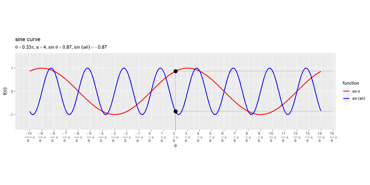
次は、sin関数の変数$\theta$の係数と周期(波長)の関係を可視化します。
グラフの作成
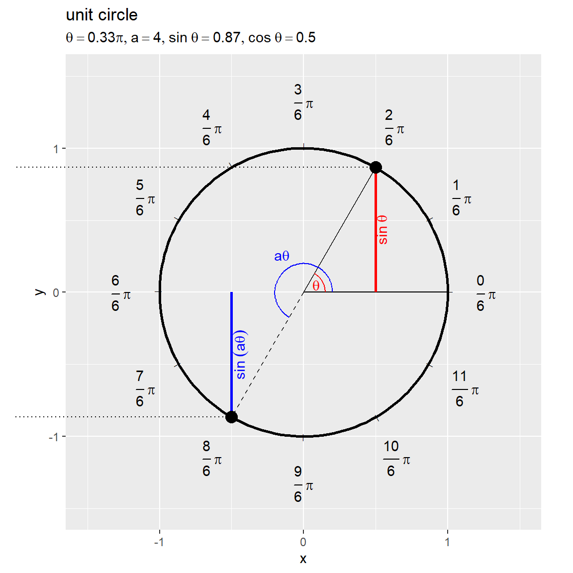
角度$\theta$を固定した$\sin(a \theta)$をグラフで確認します。
変数の係数と角度を指定します。
# 変数の係数を指定
a <- 4

# 角度を指定
alpha <- 60

# ラジアンに変換
theta <- alpha / 180 * pi
theta
## [1] 1.047198
sin関数の変数(角度)の係数$a$と、角度(ラジアン)$\theta$を指定します。
・コード(クリックで展開)
曲線上に関数の点を描画するためのデータフレームを作成します。
# 関数の点の描画用
point_df <- tibble::tibble(
  theta = c(theta, theta),
  sin_theta = sin(theta * c(1, a)),
  cos_theta = cos(theta * c(1, a)),
  fnc = c("sin theta", "sin(a theta)")
)
point_df
## # A tibble: 2 × 4
##   theta sin_theta cos_theta fnc
##   <dbl>     <dbl>     <dbl> <chr>
## 1  1.05     0.866     0.5   sin theta
## 2  1.05    -0.866    -0.500 sin(a theta)
sin関数$\sin \theta$とa倍した変数によるsin関数$\sin (a \theta)$、cos関数$\cos \theta$とa倍した変数によるcos関数$\cos(a \theta)$を計算して、$\theta$と共に格納します。
作図時の色分けなど用に、元の関数とa倍した変数による値を区別するための列fncを作成します。
単位円を描画するためのデータフレームを作成します。
# 単位円の描画用
circle_df <- tibble::tibble(
  theta = seq(from = 0, to = 2*pi, by = 0.04),
  sin_theta = sin(theta),
  cos_theta = cos(theta)
)

# 角度目盛の描画用
tick_df <- tibble::tibble(
  alpha = 0:11 * 30,
  theta = 0:11 / 6 * pi,
  x = cos(theta),
  y = sin(theta),
  rad_label = paste0("frac(", 0:11, ", 6)~pi")
)
circle_df
## # A tibble: 158 × 3
##    theta sin_theta cos_theta
##    <dbl>     <dbl>     <dbl>
##  1  0       0          1
##  2  0.04    0.0400     0.999
##  3  0.08    0.0799     0.997
##  4  0.12    0.120      0.993
##  5  0.16    0.159      0.987
##  6  0.2     0.199      0.980
##  7  0.24    0.238      0.971
##  8  0.28    0.276      0.961
##  9  0.32    0.315      0.949
## 10  0.36    0.352      0.936
## # … with 148 more rows
単位円の作図用のラジアン$0 \leq \theta \leq 2 \pi$を作成して、$\sin \theta, \cos \theta$を計算します。
tick_dfは、「関数をk倍する場合」と同じ処理です。
角度を表示するためのデータフレームを作成します。
# 半径の描画用
radius_df <- tibble::tibble(
  x_from = c(0, 0, 0),
  y_from = c(0, 0, 0),
  x_to = c(1, cos(theta), cos(theta*a)),
  y_to = c(0, sin(theta), sin(theta*a)),
  fnc = c("r", "sin theta", "sin(a theta)")
)

# 角度マークの描画用
d1 <- 0.15
d2 <- 0.2
tmp_vals  <- seq(from = min(0, theta), to = max(0, theta), length.out = 100)
angle_df <- tibble::tibble(
  rad = c(tmp_vals, tmp_vals),
  x = c(cos(tmp_vals)*d1, cos(tmp_vals*a)*d2),
  y = c(sin(tmp_vals)*d1, sin(tmp_vals*a)*d2),
  ang = c(rep(c("theta", "a theta"), each = length(tmp_vals)))
)

# 角度ラベルの描画用
d1 <- 0.1
d2 <- 0.3
angle_label_df <- tibble::tibble(
  rad = c(median(c(0, theta)), median(c(0, theta*a))),
  x = cos(rad) * c(d1, d2),
  y = sin(rad) * c(d1, d2),
  angle_label = c("theta", "a*theta"),
  ang = c("theta", "a theta")
)
radius_df; angle_df; angle_label_df
## # A tibble: 3 × 5
##   x_from y_from   x_to   y_to fnc
##    <dbl>  <dbl>  <dbl>  <dbl> <chr>
## 1      0      0  1      0     r
## 2      0      0  0.5    0.866 sin theta
## 3      0      0 -0.500 -0.866 sin(a theta)
## # A tibble: 200 × 4
##       rad     x       y ang
##     <dbl> <dbl>   <dbl> <chr>
##  1 0      0.15  0       theta
##  2 0.0106 0.150 0.00159 theta
##  3 0.0212 0.150 0.00317 theta
##  4 0.0317 0.150 0.00476 theta
##  5 0.0423 0.150 0.00634 theta
##  6 0.0529 0.150 0.00793 theta
##  7 0.0635 0.150 0.00951 theta
##  8 0.0740 0.150 0.0111  theta
##  9 0.0846 0.149 0.0127  theta
## 10 0.0952 0.149 0.0143  theta
## # … with 190 more rows
## # A tibble: 2 × 5
##     rad       x     y angle_label ang
##   <dbl>   <dbl> <dbl> <chr>       <chr>
## 1 0.524  0.0866 0.05  theta       theta
## 2 2.09  -0.15   0.260 a*theta     a theta
$0^{\circ}, \theta, a \theta$のそれぞれの角度における半径を描画するために、原点と単位円上の点を結ぶ線分の座標を格納してradius_dfとします。始点の座標をx_from, y_from、終点の座標をx_to, y_to列とします。
2つの扇形(角度マーク)を描画するための値(ラジアン)を作成して、x軸とy軸の値を計算してangle_dfとします。角度$\theta$として$0$から$\theta$、角度$a \theta$として$0$から$a \theta$の値を使います。
角度の中点に配置するように座標とラベル用の文字列を格納してangle_label_dfとします。
単位円におけるsin関数の値を描画するためのデータフレームを作成します。
# sin関数の線の描画用
sin_line_df <- tibble::tibble(
  x_from = c(cos(theta), cos(theta*a)),
  y_from = c(0, 0),
  x_to = c(cos(theta), cos(theta*a)),
  y_to = c(sin(theta), sin(theta*a)),
  fnc = c("sin theta", "sin(a theta)")
)

# sin関数の線ラベルの描画用
sin_label_df <- sin_line_df |>
  dplyr::group_by(fnc) |> # 中点の計算用
  dplyr::mutate(
    # 中点に配置
    x = median(c(x_from, x_to)),
    y = median(c(y_from, y_to))
  ) |>
  dplyr::ungroup() |>
  tibble::add_column(
    fnc_label = c("sin~theta", "sin~(a*theta)")
  ) |>
  dplyr::select(x, y, fnc, fnc_label)
sin_line_df; sin_label_df
## # A tibble: 2 × 5
##   x_from y_from   x_to   y_to fnc
##    <dbl>  <dbl>  <dbl>  <dbl> <chr>
## 1  0.5        0  0.5    0.866 sin theta
## 2 -0.500      0 -0.500 -0.866 sin(a theta)
## # A tibble: 2 × 4
##        x      y fnc          fnc_label
##    <dbl>  <dbl> <chr>        <chr>
## 1  0.5    0.433 sin theta    sin~theta
## 2 -0.500 -0.433 sin(a theta) sin~(a*theta)
これまでと同様に処理します。
単位円上の点とsin関数上の点を結ぶ線(の半分)を描画するためのデータフレームを作成します。
# 描画領域のサイズを設定
axis_size <- 1.5
l         <- 0.5

# サイン波との対応用
segment_circle_df <- tibble::tibble(
  x_from = c(cos(theta), cos(theta*a)),
  y_from = c(sin(theta), sin(theta*a)),
  x_to = c(-axis_size-l, -axis_size-l),
  y_to = c(sin(theta), sin(theta*a)),
  fnc = c("sin theta", "sin(a theta)")
)
segment_circle_df
## # A tibble: 2 × 5
##   x_from y_from  x_to   y_to fnc
##    <dbl>  <dbl> <dbl>  <dbl> <chr>
## 1  0.5    0.866    -2  0.866 sin theta
## 2 -0.500 -0.866    -2 -0.866 sin(a theta)
これまでと同様に処理します。
単位円のグラフを作成します。
# 関数ラベルを作成
fnc_label <- paste0(
  "list(",
  "theta==", round(theta/pi, digits = 2), "*pi",
  ", a==", round(a, digits = 2),
  ", sin~theta==", round(sin(theta), digits = 2),
  ", cos~theta==", round(cos(theta), digits = 2),
  ")"
)

# 円を作図
d <- 1.2
circle_graph <- ggplot() +
  geom_path(data = circle_df,
            mapping = aes(x = cos_theta, y = sin_theta),
            size = 1) + # 単位円
  geom_text(data = tick_df,
            mapping = aes(x = x, y = y, angle = alpha+90),
            label = "|", size = 2) + # 角度目盛
  geom_text(data = tick_df,
            mapping = aes(x = x*d, y = y*d, label = rad_label,
                          hjust = 1-(x*0.5+0.5), vjust = 1-(y*0.5+0.5)), parse = TRUE) + # 角度目盛ラベル
  geom_segment(data = radius_df,
               mapping = aes(x = x_from, y = y_from, xend = x_to, yend = y_to, linetype = fnc)) + # 半径
  geom_path(data = angle_df,
            mapping = aes(x = x, y = y, color = ang)) + # 角度マーク
  geom_text(data = angle_label_df,
            mapping = aes(x = x, y = y, label = angle_label, color = ang), parse = TRUE) + # 角度ラベル
  geom_segment(data = sin_line_df,
               mapping = aes(x = x_from, y = y_from, xend = x_to, yend = y_to, color = fnc),
               size = 1) + # sin関数
  geom_text(data = sin_label_df,
             mapping = aes(x = x, y = y, label = fnc_label, color = fnc), parse = TRUE,
             angle = 90, vjust = 1) + # sin関数ラベル
  geom_segment(data = segment_circle_df,
               mapping = aes(x = x_from, y = y_from, xend = x_to, yend = y_to),
               linetype = "dotted") + # sin波との対応線
  geom_point(data = point_df,
             mapping = aes(x = cos_theta, y = sin_theta),
             size = 4) + # 円上の点
  scale_color_manual(breaks = c("sin theta", "sin(a theta)", "theta", "a theta"),
                     values = c("red", "blue", "red", "blue")) + # 線の色
  scale_linetype_manual(breaks = c("sin theta", "sin(a theta)", "r"),
                        values = c("solid", "dashed", "solid")) +
  theme(legend.position = "none") + # 凡例の非表示
  coord_fixed(ratio = 1, clip = "off",
              xlim = c(-axis_size, axis_size), ylim = c(-axis_size, axis_size)) + # 描画領域
  labs(title = "unit circle",
       subtitle = parse(text = fnc_label),
       x = "x", y = "y")
circle_graph
これまでと同様に処理します。
サイン波の作図用のラジアンの値を作成します。
# 作図用のラジアンの値を作成
theta_vals <- seq(from = theta-2*pi, to = theta+2*pi, by = 0.01)
この例では、2周期分の値を指定します。
サイン波の描画するためのデータフレームを作成します。
# サイン波の描画用
sin_curve_df <- tibble::tibble(
  theta = c(theta_vals, theta_vals),
  sin_theta = c(sin(theta_vals), sin(theta_vals*a)),
  fnc = rep(c("sin theta", "sin(a theta)"), each = length(theta_vals))
)
sin_curve_df
## # A tibble: 2,514 × 3
##    theta sin_theta fnc
##    <dbl>     <dbl> <chr>
##  1 -5.24     0.866 sin theta
##  2 -5.23     0.871 sin theta
##  3 -5.22     0.876 sin theta
##  4 -5.21     0.881 sin theta
##  5 -5.20     0.885 sin theta
##  6 -5.19     0.890 sin theta
##  7 -5.18     0.894 sin theta
##  8 -5.17     0.899 sin theta
##  9 -5.16     0.903 sin theta
## 10 -5.15     0.907 sin theta
## # … with 2,504 more rows
作図用の$\theta$の値と$\sin \theta, \sin(a \theta)$の値を格納します。
先ほどと同様に、sin関数上の点と円周上の点を結ぶ線(の半分)を描画するためのデータフレームを作成します。
# x軸(角度)・単位円との対応用
d <- 1.1
segment_sin_df <- tibble::tibble(
  x_from = c(theta, theta, theta, theta),
  y_from = c(sin(theta), sin(theta), sin(theta*a), sin(theta*a)),
  x_to = c(theta, max(theta_vals)+l, theta, max(theta_vals)+l),
  y_to = c(-axis_size*d, sin(theta), -axis_size*d, sin(theta*a)),
  fnc = rep(c("sin theta", "sin(a theta)"), each = 2)
)
segment_sin_df
## # A tibble: 4 × 5
##   x_from y_from  x_to   y_to fnc
##    <dbl>  <dbl> <dbl>  <dbl> <chr>
## 1   1.05  0.866  1.05 -1.65  sin theta
## 2   1.05  0.866  7.82  0.866 sin theta
## 3   1.05 -0.866  1.05 -1.65  sin(a theta)
## 4   1.05 -0.866  7.82 -0.866 sin(a theta)
曲線上の点からx軸・y軸への垂線を引くように座標を指定します。
x軸目盛として、角度ラベルを描画するのに用いるベクトルを作成します。
# x軸目盛ラベルの描画用の値を作成
tick_min <- floor(min(theta_vals) * 6 / pi)
tick_vec <- seq(from = tick_min, to = tick_min+25, by = 1)
「関数をk倍する場合」と同じ処理です。
サイン波のグラフを作成します。
# 関数ラベルを作成
fnc_label <- paste0(
  "list(",
  "theta==", round(theta/pi, digits = 2), "*pi",
  ", a==", round(a, digits = 2),
  ", sin~theta==", round(sin(theta), digits = 2),
  ", sin~(a*theta)==", round(sin(theta*a), digits = 2),
  ")"
)

# サイン波を作図
sin_graph <- ggplot() +
  geom_line(data = sin_curve_df,
            mapping = aes(x = theta, y = sin_theta, color = fnc),
            size = 1) + # sin関数
  geom_segment(data = segment_sin_df,
               mapping = aes(x = x_from, y = y_from, xend = x_to, yend = y_to),
               linetype = "dotted") + # 単位円との対応線
  geom_point(data = point_df,
             mapping = aes(x = theta, y = sin_theta),
             size = 4) + # 関数曲線上の点
  scale_x_continuous(breaks = tick_vec/6*pi,
                     labels = parse(text = paste0("frac(", tick_vec, ", 6)~pi"))) + # 角度目盛ラベル
  scale_color_manual(breaks = c("sin theta", "sin(a theta)"),
                     values = c("red", "blue"),
                     labels = parse(text = c("sin~theta", "sin~(a*theta)")),
                     name = "function") + # 線の色
  theme(legend.text.align = 0) + # 凡例の設定
  coord_fixed(ratio = 1, clip = "off",
              xlim = c(min(theta_vals), max(theta_vals)), ylim = c(-axis_size, axis_size)) + # 描画領域
  labs(title = "sine curve",
       subtitle = parse(text = fnc_label),
       x = expression(theta), y = expression(f(theta)))
sin_graph
「関数をk倍する場合」と同様に処理します。
2つのグラフを並べて描画します。
# グラフを並べて描画
patchwork::wrap_plots(sin_graph, circle_graph) +
  patchwork::plot_layout(guides = "collect")
・$\theta^{\circ} = 120^{\circ}, a = 4$のグラフ
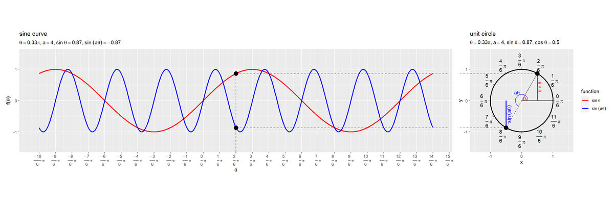
角度$\theta$が$a$倍になることで、角速度(角の変化)も$a$倍になります。よって、波長が$\frac{1}{a}$倍($2 \pi$の範囲での周期の数が$a$倍)になるのを確認できます。
・$\theta^{\circ} = 120^{\circ}, a = -1$のグラフ
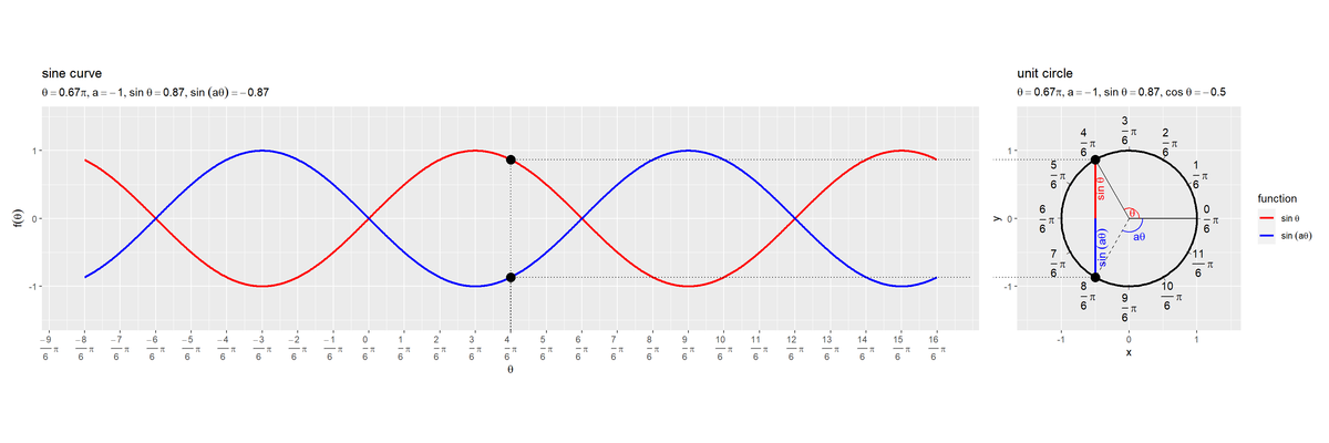
$a$が負の値のとき、$x = 0$の直線に対して反転したグラフになります。
$a = -1$のとき、「関数をk倍する場合」の$k = -1$のときや「変数にbを加える場合」の$b = \pi$のとき、サイン波の形が同じになりますが、単位円の点(単位円における位置関係)が異なるのが分かります。
アニメーションの作成
続いて、角度を変化させたアニメーションで確認します。
フレーム数と角度の範囲を指定して、角度として用いる値を作成します。
# フレーム数を指定
frame_num <- 100

# 変数の定数項を指定
a <- 2

# 角度の範囲を指定
theta_min <- -2 * pi
theta_max <- 2 * pi

# フレームごとの角度を作成
theta_i <- seq(from = theta_min, to = theta_max, length.out = frame_num+1)[1:frame_num]
「関数をk倍する場合」と同じ処理です。
・コード(クリックで展開)
theta_iから順番に値を取り出して作図し、グラフを書き出します
# 一時保存フォルダを指定
dir_path <- "tmp_folder"

# 描画領域のサイズを設定
axis_size <- 1.5
l         <- 0.6

# 角度ごとに作図
for(i in 1:frame_num) {

  # i番目の角度を取得
  theta <- theta_i[i]

  # 関数の点の描画用
  point_df <- tibble::tibble(
    theta = c(theta, theta),
    sin_theta = sin(theta * c(1, a)),
    cos_theta = cos(theta * c(1, a)),
    fnc = c("sin theta", "sin(a theta)")
  )

  # 半径の描画用
  radius_df <- tibble::tibble(
    x_from = c(0, 0, 0),
    y_from = c(0, 0, 0),
    x_to = c(1, cos(theta), cos(theta*a)),
    y_to = c(0, sin(theta), sin(theta*a)),
    fnc = c("r", "sin theta", "sin(a theta)")
  )

  # 角度マークの描画用
  d1 <- 0.15
  d2 <- 0.2
  tmp_vals  <- seq(from = min(0, theta), to = max(0, theta), length.out = 100)
  angle_df <- tibble::tibble(
    rad = c(tmp_vals, tmp_vals),
    x = c(cos(tmp_vals)*d1, cos(tmp_vals*a)*d2),
    y = c(sin(tmp_vals)*d1, sin(tmp_vals*a)*d2),
    ang = c(rep(c("theta", "a theta"), each = length(tmp_vals)))
  )

  # 角度ラベルの描画用
  d1 <- 0.1
  d2 <- 0.3
  angle_label_df <- tibble::tibble(
    rad = c(median(c(0, theta)), median(c(0, theta*a))),
    x = cos(rad) * c(d1, d2),
    y = sin(rad) * c(d1, d2),
    angle_label = c("theta", "a*theta"),
    ang = c("theta", "a theta")
  )

  # sin関数の線の描画用
  sin_line_df <- tibble::tibble(
    x_from = c(cos(theta), cos(theta*a)),
    y_from = c(0, 0),
    x_to = c(cos(theta), cos(theta*a)),
    y_to = c(sin(theta), sin(theta*a)),
    fnc = c("sin theta", "sin(a theta)")
  )

  # sin関数の線ラベルの描画用
  sin_label_df <- sin_line_df |>
    dplyr::group_by(fnc) |> # 中点の計算用
    dplyr::mutate(
      # 中点に配置
      x = median(c(x_from, x_to)),
      y = median(c(y_from, y_to))
    ) |>
    dplyr::ungroup() |>
    tibble::add_column(
      fnc_label = c("sin~theta", "sin~(a*theta)")
    ) |>
    dplyr::select(x, y, fnc, fnc_label)

  # サイン波との対応用
  segment_circle_df <- tibble::tibble(
    x_from = c(cos(theta), cos(theta*a)),
    y_from = c(sin(theta), sin(theta*a)),
    x_to = c(-axis_size-l, -axis_size-l),
    y_to = c(sin(theta), sin(theta*a)),
    fnc = c("sin theta", "sin(a theta)")
  )

  # 関数ラベルを作成
  fnc_label <- paste0(
    "list(",
    "theta==", round(theta/pi, digits = 2), "*pi",
    ", a==", round(a, digits = 2),
    ", sin~theta==", round(sin(theta), digits = 2),
    ", cos~theta==", round(cos(theta), digits = 2),
    ")"
  )

  # 円を作図
  d <- 1.2
  circle_graph <- ggplot() +
    geom_path(data = circle_df,
              mapping = aes(x = cos_theta, y = sin_theta),
              size = 1) + # 単位円
    geom_text(data = tick_df,
              mapping = aes(x = x, y = y, angle = alpha+90),
              label = "|", size = 2) + # 角度目盛
    geom_text(data = tick_df,
              mapping = aes(x = x*d, y = y*d, label = rad_label,
                            hjust = 1-(x*0.5+0.5), vjust = 1-(y*0.5+0.5)), parse = TRUE) + # 角度目盛ラベル
    geom_segment(data = radius_df,
                 mapping = aes(x = x_from, y = y_from, xend = x_to, yend = y_to, linetype = fnc)) + # 半径
    geom_path(data = angle_df,
              mapping = aes(x = x, y = y, color = ang)) + # 角度マーク
    geom_text(data = angle_label_df,
              mapping = aes(x = x, y = y, label = angle_label, color = ang), parse = TRUE) + # 角度ラベル
    geom_segment(data = sin_line_df,
                 mapping = aes(x = x_from, y = y_from, xend = x_to, yend = y_to, color = fnc),
                 size = 1) + # sin関数
    geom_text(data = sin_label_df,
               mapping = aes(x = x, y = y, label = fnc_label, color = fnc), parse = TRUE,
               angle = 90, vjust = 1) + # sin関数ラベル
    geom_segment(data = segment_circle_df,
                 mapping = aes(x = x_from, y = y_from, xend = x_to, yend = y_to),
                 linetype = "dotted") + # sin波との対応線
    geom_point(data = point_df,
               mapping = aes(x = cos_theta, y = sin_theta),
               size = 4) + # 円上の点
    scale_color_manual(breaks = c("sin theta", "sin(a theta)", "theta", "a theta"),
                       values = c("red", "blue", "red", "blue")) + # 線の色
    scale_linetype_manual(breaks = c("sin theta", "sin(a theta)", "r"),
                          values = c("solid", "dashed", "solid")) +
    theme(legend.position = "none") + # 凡例の非表示
    coord_fixed(ratio = 1, clip = "off",
                xlim = c(-axis_size, axis_size), ylim = c(-axis_size, axis_size)) + # 描画領域
    labs(title = "unit circle",
         subtitle = parse(text = fnc_label),
         x = "x", y = "y")

  # 作図用のラジアンの値を作成
  theta_size <- 2 * pi
  theta_vals <- seq(from = max(theta_min, theta-theta_size), to = theta, by = 0.01)

  # サイン波の描画用
  sin_curve_df <- tibble::tibble(
    theta = c(theta_vals, theta_vals),
    sin_theta = c(sin(theta_vals), sin(theta_vals*a)),
    fnc = rep(c("sin theta", "sin(a theta)"), each = length(theta_vals))
  )

  # x軸(角度)・単位円との対応用
  d <- 1.1
  segment_sin_df <- tibble::tibble(
    x_from = c(theta, theta, theta, theta),
    y_from = c(sin(theta), sin(theta), sin(theta*a), sin(theta*a)),
    x_to = c(theta, max(theta_vals)+l, theta, max(theta_vals)+l),
    y_to = c(-axis_size*d, sin(theta), -axis_size*d, sin(theta*a)),
    fnc = rep(c("sin theta", "sin(a theta)"), each = 2)
  )

  # x軸目盛ラベルの描画用の値を作成
  tick_min <- floor((theta-theta_size) * 6 / pi)
  tick_vec <- seq(from = tick_min, to = tick_min+13, by = 1)

  # 関数ラベルを作成
  fnc_label <- paste0(
    "list(",
    "theta==", round(theta/pi, digits = 2), "*pi",
    ", a==", round(a, digits = 2),
    ", sin~theta==", round(sin(theta), digits = 2),
    ", sin~(a*theta)==", round(sin(theta*a), digits = 2),
    ")"
  )

  # サイン波を作図
  sin_graph <- ggplot() +
    geom_line(data = sin_curve_df,
              mapping = aes(x = theta, y = sin_theta, color = fnc),
              size = 1) + # sin関数
    geom_segment(data = segment_sin_df,
                 mapping = aes(x = x_from, y = y_from, xend = x_to, yend = y_to),
                 linetype = "dotted") + # 単位円との対応線
    geom_point(data = point_df,
               mapping = aes(x = theta, y = sin_theta),
               size = 4) + # 関数曲線上の点
    scale_x_continuous(breaks = tick_vec/6*pi,
                       labels = parse(text = paste0("frac(", tick_vec, ", 6)~pi"))) + # 角度目盛ラベル
    scale_color_manual(breaks = c("sin theta", "sin(a theta)"),
                       values = c("red", "blue"),
                       labels = parse(text = c("sin~theta", "sin~(a*theta)")),
                       name = "function") + # 線の色
    theme(legend.text.align = 0) + # 凡例の設定
    coord_fixed(ratio = 1, clip = "off",
                xlim = c(theta-theta_size, theta), ylim = c(-axis_size, axis_size)) + # 描画領域
    labs(title = "sine curve",
         subtitle = parse(text = fnc_label),
         x = expression(theta), y = expression(f(theta)))

  # グラフを並べて描画
  graph <- patchwork::wrap_plots(sin_graph, circle_graph) +
      patchwork::plot_layout(guides = "collect")

  # ファイルを書き出し
  file_path <- paste0(dir_path, "/", stringr::str_pad(i, width = nchar(frame_num), pad = "0"), ".png")
  ggplot2::ggsave(filename = file_path, plot = graph, width = 1200, height = 600, units = "px", dpi = 100)

  # 途中経過を表示
  message("\r", i, "/", frame_num, appendLF = FALSE)
}
「グラフの作成」で作成したcircle_df, tick_dfも使います。
「関数をk倍する場合」のコードでgif画像を作成します。
・$a = 2$の推移
円周上($2 \pi$の範囲)を$\sin(\theta)$の点が1周する間に、$\sin(a \theta)$の点がa周するのを確認できます。
・$a = -2$の推移
$a$が負の値のとき、円周上の点が逆回転します。
・$a = -1$の推移
$k = -1$や$b = \pi$のグラフと比較します。
変数にbを加える場合
sin関数の変数$\theta$に加える定数と平行移動の関係を可視化します。
グラフの作成
角度$\theta$を固定した$\sin(\theta + b)$をグラフで確認します。
変数に加える定数と角度を指定します。
# 変数の定数項を指定
b <- 0.5 * pi

# 角度を指定
alpha <- 120

# ラジアンに変換
theta <- alpha / 180 * pi
theta
## [1] 2.094395
sin関数の変数(角度)の定数項$b$と、角度(ラジアン)$\theta$を指定します。
・コード(クリックで展開)
曲線上に関数の点を描画するためのデータフレームを作成します。
# 関数の点の描画用
point_df <- tibble::tibble(
  theta = c(theta, theta),
  sin_theta = sin(theta + c(0, b)),
  cos_theta = cos(theta + c(0, b)),
  fnc = c("sin theta", "sin(theta+b)")
)
point_df
## # A tibble: 2 × 4
##   theta sin_theta cos_theta fnc
##   <dbl>     <dbl>     <dbl> <chr>
## 1  2.09     0.866    -0.5   sin theta
## 2  2.09    -0.50     -0.866 sin(theta+b)
sin関数$\sin \theta$と定数を加えた変数によるsin関数$\sin (\theta + b)$、cos関数$\cos \theta$と定数を加えた変数によるcos関数$\cos(\theta + b)$を計算して、$\theta$と共に格納します。
作図時の色分けなど用に、元の関数と定数を加えた変数による値を区別するための列fncを作成します。
単位円を描画するためのデータフレームを作成します。
# 単位円の描画用
circle_df <- tibble::tibble(
  theta = seq(from = 0, to = 2*pi, by = 0.05),
  sin_theta = sin(theta),
  cos_theta = cos(theta)
)

# 角度目盛の描画用
tick_df <- tibble::tibble(
  alpha = 0:11 * 30,
  theta = 0:11 / 6 * pi,
  x = cos(theta),
  y = sin(theta),
  rad_label = paste0("frac(", 0:11, ", 6)~pi")
)
「変数をa倍する場合」と同じ処理です。
角度を表示するためのデータフレームを作成します。
# 半径の描画用
radius_df <- tibble::tibble(
  x_from = c(0, 0, 0),
  y_from = c(0, 0, 0),
  x_to = c(1, cos(theta), cos(theta+b)),
  y_to = c(0, sin(theta), sin(theta+b)),
  fnc = c("r", "sin theta", "sin(theta+b)")
)

# 角度マークの描画用
d1 <- 0.15
d2 <- 0.2
d3 <- 0.4
tmp_t_vals  <- seq(from = min(0, theta), to = max(0, theta), length.out = 100)
tmp_b_vals  <- seq(from = min(theta, theta+b),  to = max(theta, theta+b), length.out = 100)
tmp_tb_vals <- seq(from = min(0, theta+b),  to = max(0, theta+b), length.out = 100)
angle_df <- tibble::tibble(
  rad = c(tmp_t_vals, tmp_b_vals, tmp_tb_vals),
  x = c(cos(tmp_t_vals)*d1, cos(tmp_b_vals)*d2, cos(tmp_tb_vals)*d3),
  y = c(sin(tmp_t_vals)*d1, sin(tmp_b_vals)*d2, sin(tmp_tb_vals)*d3),
  ang = c(
    rep("theta", times = length(tmp_t_vals)),
    rep("b", times = length(tmp_b_vals)),
    rep("theta+b", times = length(tmp_tb_vals))
  )
)

# 角度ラベルの描画用
d1 <- 0.1
d2 <- 0.3
d3 <- 0.5
angle_label_df <- tibble::tibble(
  rad = c(median(c(0, theta)), median(c(theta, theta+b)), median(c(0, theta+b))),
  x = cos(rad) * c(d1, d2, d3),
  y = sin(rad) * c(d1, d2, d3),
  angle_label = c("theta", "b", "(theta+b)"),
  ang = c("theta", "b", "theta+b")
)
radius_df; angle_df; angle_label_df
## # A tibble: 3 × 5
##   x_from y_from   x_to   y_to fnc
##    <dbl>  <dbl>  <dbl>  <dbl> <chr>
## 1      0      0  1      0     r
## 2      0      0 -0.5    0.866 sin theta
## 3      0      0 -0.866 -0.50  sin(theta+b)
## # A tibble: 300 × 4
##       rad     x       y ang
##     <dbl> <dbl>   <dbl> <chr>
##  1 0      0.15  0       theta
##  2 0.0212 0.150 0.00317 theta
##  3 0.0423 0.150 0.00634 theta
##  4 0.0635 0.150 0.00951 theta
##  5 0.0846 0.149 0.0127  theta
##  6 0.106  0.149 0.0158  theta
##  7 0.127  0.149 0.0190  theta
##  8 0.148  0.148 0.0221  theta
##  9 0.169  0.148 0.0253  theta
## 10 0.190  0.147 0.0284  theta
## # … with 290 more rows
## # A tibble: 3 × 5
##     rad      x      y angle_label ang
##   <dbl>  <dbl>  <dbl> <chr>       <chr>
## 1  1.05  0.05  0.0866 theta       theta
## 2  2.88 -0.290 0.0776 b           b
## 3  1.83 -0.129 0.483  (theta+b)   theta+b
$0^{\circ}, \theta, b, \theta + b$のそれぞれの角度における半径を描画するために、原点と単位円上の点を結ぶ線分の座標を格納してradius_dfとします。始点の座標をx_from, y_from、終点の座標をx_to, y_to列とします。
3つの扇形(角度マーク)を描画するための値(ラジアン)を作成して、x軸とy軸の値を計算してangle_dfとします。角度$\theta$として$0$から$\theta$、角度$b$として$\theta$から$b$、角度$\theta + b$として$0$から$\theta + b$の値を使います。
角度の中点に配置するように座標とラベル用の文字列を格納してangle_label_dfとします。
単位円におけるsin関数の値を描画するためのデータフレームを作成します。
# sin関数の線の描画用
sin_line_df <- tibble::tibble(
  x_from = c(cos(theta), cos(theta+b)),
  y_from = c(0, 0),
  x_to = c(cos(theta), cos(theta+b)),
  y_to = c(sin(theta), sin(theta+b)),
  fnc = c("sin theta", "sin(theta+b)")
)

# sin関数の線ラベルの描画用
sin_label_df <- sin_line_df |>
  dplyr::group_by(fnc) |> # 中点の計算用
  dplyr::mutate(
    # 中点に配置
    x = median(c(x_from, x_to)),
    y = median(c(y_from, y_to))
  ) |>
  dplyr::ungroup() |>
  tibble::add_column(
    fnc_label = c("sin~theta", "sin~(theta+b)")
  ) |>
  dplyr::select(x, y, fnc, fnc_label)
sin_line_df; sin_label_df
## # A tibble: 2 × 5
##   x_from y_from   x_to   y_to fnc
##    <dbl>  <dbl>  <dbl>  <dbl> <chr>
## 1 -0.5        0 -0.5    0.866 sin theta
## 2 -0.866      0 -0.866 -0.50  sin(theta+b)
## # A tibble: 2 × 4
##        x      y fnc          fnc_label
##    <dbl>  <dbl> <chr>        <chr>
## 1 -0.5    0.433 sin theta    sin~theta
## 2 -0.866 -0.25  sin(theta+b) sin~(theta+b)
これまでと同様に処理します。
単位円上の点とsin関数上の点を結ぶ線(の半分)を描画するためのデータフレームを作成します。
# 描画領域のサイズを設定
axis_size <- 1.5
l         <- 0.5

# サイン波との対応用
segment_circle_df <- tibble::tibble(
  x_from = c(cos(theta), cos(theta+b)),
  y_from = c(sin(theta), sin(theta+b)),
  x_to = c(-axis_size-l, -axis_size-l),
  y_to = c(sin(theta), sin(theta+b)),
  fnc = c("sin theta", "sin(theta+b)")
)
segment_circle_df
## # A tibble: 2 × 5
##   x_from y_from  x_to   y_to fnc
##    <dbl>  <dbl> <dbl>  <dbl> <chr>
## 1 -0.5    0.866    -2  0.866 sin theta
## 2 -0.866 -0.50     -2 -0.50  sin(theta+b)
単位円上の点からy軸への垂線を引くように座標を指定します。作図時に、隣のグラフに届かないような長さlを指定します。
また、2つのグラフの描画範囲を固定するために、axis_sizeとして値を指定しておきます。
単位円のグラフを作成します。
# 関数ラベルを作成
fnc_label <- paste0(
  "list(",
  "theta==", round(theta/pi, digits = 2), "*pi",
  ", b==", round(b, digits = 2),
  ", sin~theta==", round(sin(theta), digits = 2),
  ", cos~theta==", round(cos(theta), digits = 2),
  ")"
)

# 円を作図
d <- 1.2
circle_graph <- ggplot() +
  geom_path(data = circle_df,
            mapping = aes(x = cos_theta, y = sin_theta),
            size = 1) + # 単位円
  geom_text(data = tick_df,
            mapping = aes(x = x, y = y, angle = alpha+90),
            label = "|", size = 2) + # 角度目盛
  geom_text(data = tick_df,
            mapping = aes(x = x*d, y = y*d, label = rad_label,
                          hjust = 1-(x*0.5+0.5), vjust = 1-(y*0.5+0.5)), parse = TRUE) + # 角度目盛ラベル
  geom_segment(data = radius_df,
               mapping = aes(x = x_from, y = y_from, xend = x_to, yend = y_to, linetype = fnc)) + # 半径
  geom_path(data = angle_df,
            mapping = aes(x = x, y = y, color = ang)) + # 角度マーク
  geom_text(data = angle_label_df,
            mapping = aes(x = x, y = y, label = angle_label, color = ang), parse = TRUE) + # 角度ラベル
  geom_segment(data = sin_line_df,
               mapping = aes(x = x_from, y = y_from, xend = x_to, yend = y_to, color = fnc),
               size = 1) + # sin関数
  geom_text(data = sin_label_df,
             mapping = aes(x = x, y = y, label = fnc_label, color = fnc), parse = TRUE,
             angle = 90, vjust = 1) + # sin関数ラベル
  geom_segment(data = segment_circle_df,
               mapping = aes(x = x_from, y = y_from, xend = x_to, yend = y_to),
               linetype = "dotted") + # sin波との対応線
  geom_point(data = point_df,
             mapping = aes(x = cos_theta, y = sin_theta),
             size = 4) + # 円上の点
  scale_color_manual(breaks = c("sin theta", "sin(theta+b)", "theta", "b", "theta+b"),
                     values = c("red", "blue", "red", "purple", "blue")) + # 線の色
  scale_linetype_manual(breaks = c("sin theta", "sin(theta+b)", "r"),
                        values = c("solid", "dashed", "solid")) +
  theme(legend.position = "none") + # 凡例の非表示
  coord_fixed(ratio = 1, clip = "off",
              xlim = c(-axis_size, axis_size), ylim = c(-axis_size, axis_size)) + # 描画領域
  labs(title = "unit circle",
       subtitle = parse(text = fnc_label),
       x = "x", y = "y")
circle_graph
これまでと同様に処理します。
サイン波の作図用のラジアンの値を作成します。
# 作図用のラジアンの値を作成
theta_vals <- seq(from = theta-2*pi, to = theta+2*pi, by = 0.01)
この例では、2周期分の値を指定します。
サイン波の描画するためのデータフレームを作成します。
# サイン波の描画用
sin_curve_df <- tibble::tibble(
  theta = c(theta_vals, theta_vals),
  sin_theta = c(sin(theta_vals), sin(theta_vals+b)),
  fnc = rep(c("sin theta", "sin(theta+b)"), each = length(theta_vals))
)
sin_curve_df
## # A tibble: 2,514 × 3
##    theta sin_theta fnc
##    <dbl>     <dbl> <chr>
##  1 -4.19     0.866 sin theta
##  2 -4.18     0.861 sin theta
##  3 -4.17     0.856 sin theta
##  4 -4.16     0.851 sin theta
##  5 -4.15     0.845 sin theta
##  6 -4.14     0.840 sin theta
##  7 -4.13     0.834 sin theta
##  8 -4.12     0.829 sin theta
##  9 -4.11     0.823 sin theta
## 10 -4.10     0.818 sin theta
## # … with 2,504 more rows
作図用の$\theta$の値と$\sin \theta, \sin(\theta + b)$の値を格納します。
先ほどと同様に、sin関数上の点と円周上の点を結ぶ線(の半分)を描画するためのデータフレームを作成します。
# x軸(角度)・単位円との対応用
d <- 1.1
segment_sin_df <- tibble::tibble(
  x_from = c(theta, theta, theta, theta),
  y_from = c(sin(theta), sin(theta), sin(theta+b), sin(theta+b)),
  x_to = c(theta, max(theta_vals)+l, theta, max(theta_vals)+l),
  y_to = c(-axis_size*d, sin(theta), -axis_size*d, sin(theta+b)),
  fnc = rep(c("sin theta", "sin(theta+b)"), each = 2)
)
segment_sin_df
## # A tibble: 4 × 5
##   x_from y_from  x_to   y_to fnc
##    <dbl>  <dbl> <dbl>  <dbl> <chr>
## 1   2.09  0.866  2.09 -1.65  sin theta
## 2   2.09  0.866  8.87  0.866 sin theta
## 3   2.09 -0.50   2.09 -1.65  sin(theta+b)
## 4   2.09 -0.50   8.87 -0.50  sin(theta+b)
曲線上の点からx軸・y軸への垂線を引くように座標を指定します。
角度$b$に関して描画するためのデータフレームを作成します。
# 角度bに関する可視化用
b_df <- tibble::tibble(
  x = theta+b,
  y = sin(theta+b),
  x_to = theta,
  y_to = sin(theta+b),
  angle_lable = "b"
) |>
  dplyr::mutate(
    # 中点に配置
    x_mid = median(c(x, x_to)),
    y_mid = median(c(y, y_to))
  )
b_df
## # A tibble: 1 × 7
##       x     y  x_to  y_to angle_lable x_mid y_mid
##   <dbl> <dbl> <dbl> <dbl> <chr>       <dbl> <dbl>
## 1  3.67 -0.50  2.09 -0.50 b            2.88 -0.50
角度$\theta + b$における点の座標をx, y列、角度$\theta$における点の座標をx_to, y_to列、またその中点をx_mid, y_mid列として、ラベル用の文字列と共に格納します。
x軸目盛として、角度ラベルを描画するのに用いるベクトルを作成します。
# x軸目盛ラベルの描画用の値を作成
tick_min <- floor(min(theta_vals) * 6 / pi)
tick_vec <- seq(from = tick_min, to = tick_min+25, by = 1)
「関数をk倍する場合」と同じ処理です。
サイン波のグラフを作成します。
# 関数ラベルを作成
fnc_label <- paste0(
  "list(",
  "theta==", round(theta/pi, digits = 2), "*pi",
  ", b==", round(b, digits = 2),
  ", sin~theta==", round(sin(theta), digits = 2),
  ", sin~(theta+b)==", round(sin(theta+b), digits = 2),
  ")"
)

# サイン波を作図
sin_graph <- ggplot() +
  geom_line(data = sin_curve_df,
            mapping = aes(x = theta, y = sin_theta, color = fnc),
            size = 1) + # sin関数
  geom_segment(data = segment_sin_df,
               mapping = aes(x = x_from, y = y_from, xend = x_to, yend = y_to),
               linetype = "dotted") + # 単位円との対応線
  geom_segment(data = b_df,
               mapping = aes(x = x, y = y, xend = x_to, yend = y_to),
               color ="purple") + # 長さbの線分
  geom_text(data = b_df,
            mapping = aes(x = x_mid, y = y_mid, label = angle_lable),
            vjust = -0.5, color = "purple") + # 線分bのラベル
  geom_point(data = b_df,
             mapping = aes(x = x, y = y),
             size = 4, shape = 1) + # theta+bの点
  geom_point(data = point_df,
             mapping = aes(x = theta, y = sin_theta),
             size = 4) + # 関数曲線上の点
  scale_x_continuous(breaks = tick_vec/6*pi,
                     labels = parse(text = paste0("frac(", tick_vec, ", 6)~pi"))) + # 角度目盛ラベル
  scale_color_manual(breaks = c("sin theta", "sin(theta+b)"),
                     values = c("red", "blue"),
                     labels = parse(text = c("sin~theta", "sin~(theta+b)")),
                     name = "function") + # 線の色
  theme(legend.text.align = 0) + # 凡例の設定
  coord_fixed(ratio = 1, clip = "off",
              xlim = c(min(theta_vals), max(theta_vals)), ylim = c(-axis_size, axis_size)) + # 描画領域
  labs(title = "sine curve",
       subtitle = parse(text = fnc_label),
       x = expression(theta), y = expression(f(theta)))
sin_graph
「関数をk倍する場合」の作図処理に、角度$b$に関しても可視化します。
2つのグラフを並べて描画します。
# グラフを並べて描画
patchwork::wrap_plots(sin_graph, circle_graph) +
  patchwork::plot_layout(guides = "collect")
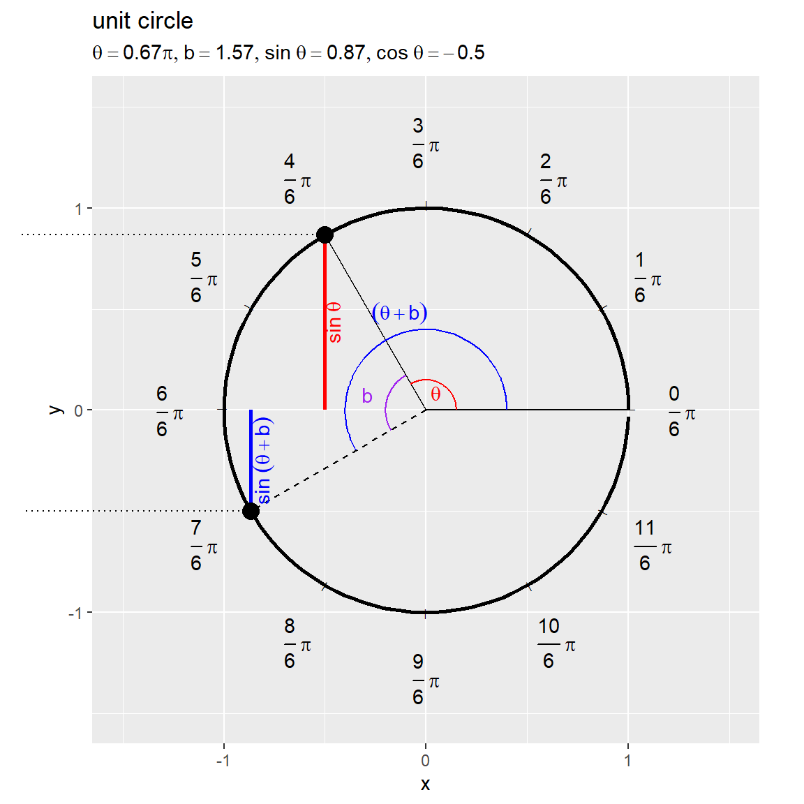
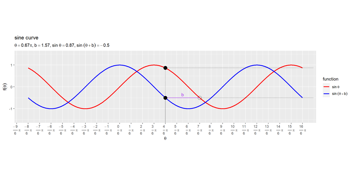
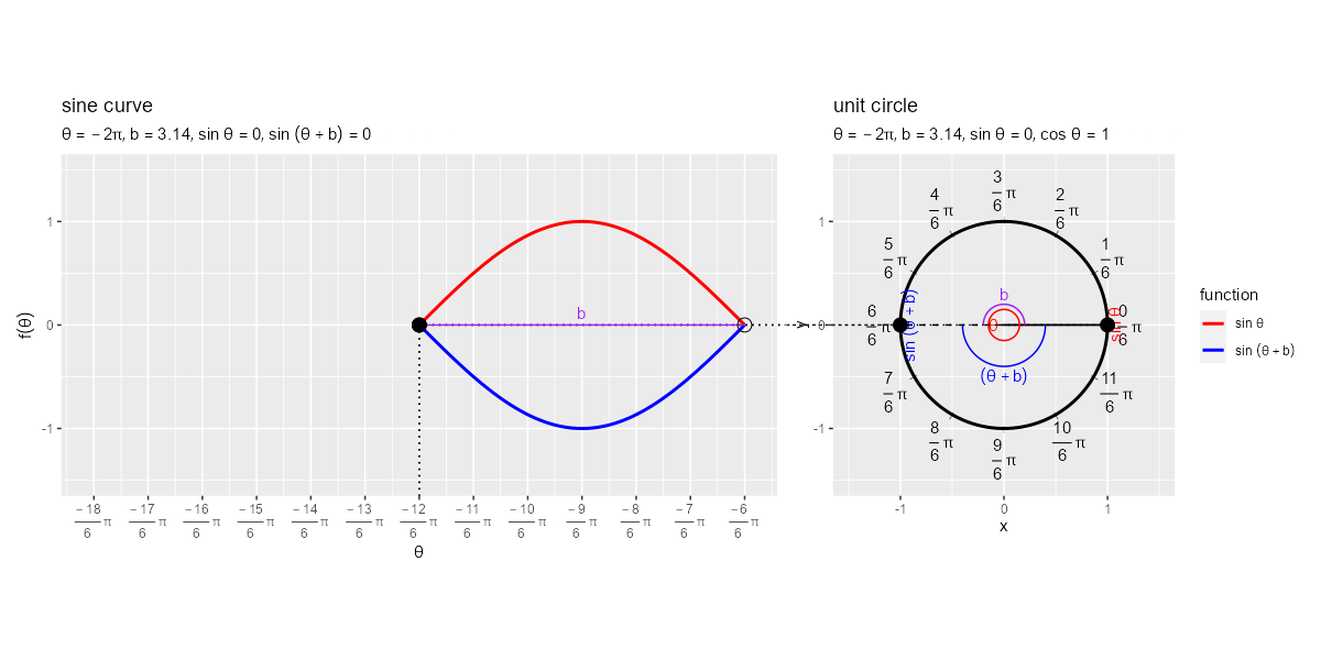
・$\theta^{\circ} = 120^{\circ}, b = \frac{1}{2} \pi$のグラフ
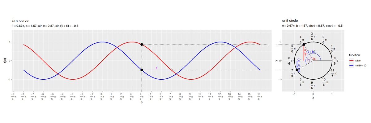
角度$\theta$の曲線(赤色の線)に角度$b$が加えられることで、角度$\theta + b$の曲線(青色の線)が、x軸方向に$-b$(紫色の直線)だけ平行移動する($b$の分戻る)のを確認できます。
・$\theta^{\circ} = 120^{\circ}, b = -\frac{1}{2} \pi$のグラフ
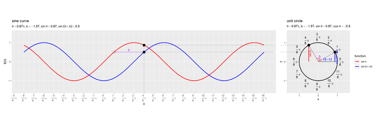
$b$が負の値の(変数から定数を引いた)場合は、x軸方向に$b$だけ平行移動する($b$の分進む)のを確認できます。
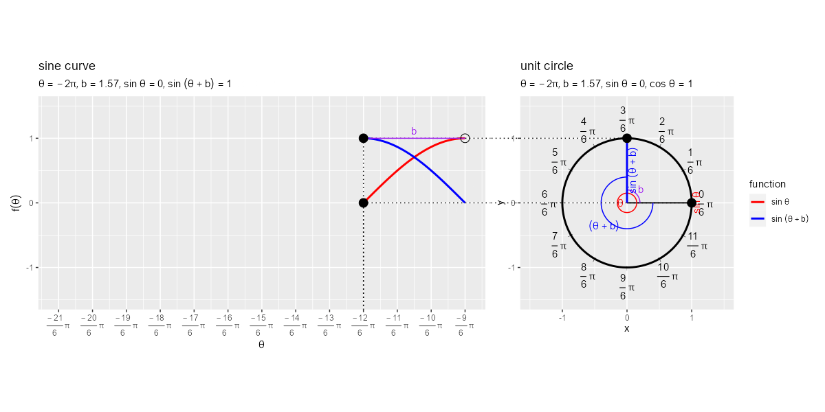
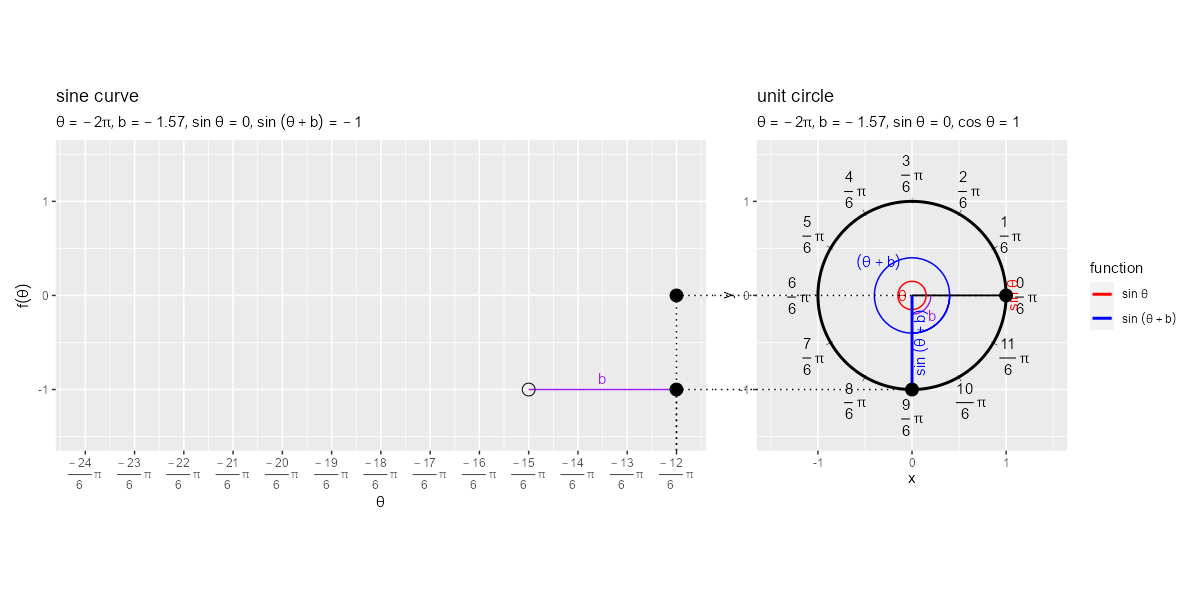
・$\theta^{\circ} = 120^{\circ}, b = \pi$のグラフ

「関数をk倍する場合」の$k = -1$のときと同じグラフになるのを確認できます。
アニメーションの作成
続いて、角度を変化させたアニメーションで確認します。
フレーム数と角度の範囲を指定して、角度として用いる値を作成します。
# フレーム数を指定
frame_num <- 100

# 変数の定数項を指定
b <- -0.5 * pi

# 角度の範囲を指定
theta_min <- -2 * pi
theta_max <- 2 * pi

# フレームごとの角度を作成
theta_i <- seq(from = theta_min, to = theta_max, length.out = frame_num+1)[1:frame_num]
「関数をk倍する場合」と同じ処理です。
・コード(クリックで展開)
theta_iから順番に値を取り出して作図し、グラフを書き出します
# 一時保存フォルダを指定
dir_path <- "tmp_folder"

# 描画領域のサイズを設定
axis_size <- 1.5
l         <- 0.6

# 角度ごとに作図
for(i in 1:frame_num) {

  # i番目の角度を取得
  theta <- theta_i[i]

  # 関数の点の描画用
  point_df <- tibble::tibble(
    theta = c(theta, theta),
    sin_theta = sin(theta + c(0, b)),
    cos_theta = cos(theta + c(0, b)),
    fnc = c("sin theta", "sin(theta+b)")
  )

  # 半径の描画用
  radius_df <- tibble::tibble(
    x_from = c(0, 0, 0),
    y_from = c(0, 0, 0),
    x_to = c(1, cos(theta), cos(theta+b)),
    y_to = c(0, sin(theta), sin(theta+b)),
    fnc = c("r", "sin theta", "sin(theta+b)")
  )

  # 角度マークの描画用
  d1 <- 0.15
  d2 <- 0.2
  d3 <- 0.4
  tmp_t_vals  <- seq(from = min(0, theta), to = max(0, theta), length.out = 100)
  tmp_b_vals  <- seq(from = min(theta, theta+b),  to = max(theta, theta+b), length.out = 100)
  tmp_tb_vals <- seq(from = min(0, theta+b),  to = max(0, theta+b), length.out = 100)
  angle_df <- tibble::tibble(
    rad = c(tmp_t_vals, tmp_b_vals, tmp_tb_vals),
    x = c(cos(tmp_t_vals)*d1, cos(tmp_b_vals)*d2, cos(tmp_tb_vals)*d3),
    y = c(sin(tmp_t_vals)*d1, sin(tmp_b_vals)*d2, sin(tmp_tb_vals)*d3),
    ang = c(
      rep("theta", times = length(tmp_t_vals)),
      rep("b", times = length(tmp_b_vals)),
      rep("theta+b", times = length(tmp_tb_vals))
    )
  )

  # 角度ラベルの描画用
  d1 <- 0.1
  d2 <- 0.3
  d3 <- 0.5
  angle_label_df <- tibble::tibble(
    rad = c(median(c(0, theta)), median(c(theta, theta+b)), median(c(0, theta+b))),
    x = cos(rad) * c(d1, d2, d3),
    y = sin(rad) * c(d1, d2, d3),
    angle_label = c("theta", "b", "(theta+b)"),
    ang = c("theta", "b", "theta+b")
  )

  # sin関数の線の描画用
  sin_line_df <- tibble::tibble(
    x_from = c(cos(theta), cos(theta+b)),
    y_from = c(0, 0),
    x_to = c(cos(theta), cos(theta+b)),
    y_to = c(sin(theta), sin(theta+b)),
    fnc = c("sin theta", "sin(theta+b)")
  )

  # sin関数の線ラベルの描画用
  sin_label_df <- sin_line_df |>
    dplyr::group_by(fnc) |> # 中点の計算用
    dplyr::mutate(
      # 中点に配置
      x = median(c(x_from, x_to)),
      y = median(c(y_from, y_to))
    ) |>
    dplyr::ungroup() |>
    tibble::add_column(
      fnc_label = c("sin~theta", "sin~(theta+b)")
    ) |>
    dplyr::select(x, y, fnc, fnc_label)

  # サイン波との対応用
  segment_circle_df <- tibble::tibble(
    x_from = c(cos(theta), cos(theta+b)),
    y_from = c(sin(theta), sin(theta+b)),
    x_to = c(-axis_size-l, -axis_size-l),
    y_to = c(sin(theta), sin(theta+b)),
    fnc = c("sin theta", "sin(theta+b)")
  )

  # 関数ラベルを作成
  fnc_label <- paste0(
    "list(",
    "theta==", round(theta/pi, digits = 2), "*pi",
    ", b==", round(b, digits = 2),
    ", sin~theta==", round(sin(theta), digits = 2),
    ", cos~theta==", round(cos(theta), digits = 2),
    ")"
  )

  # 円を作図
  d <- 1.2
  circle_graph <- ggplot() +
    geom_path(data = circle_df,
              mapping = aes(x = cos_theta, y = sin_theta),
              size = 1) + # 単位円
    geom_text(data = tick_df,
              mapping = aes(x = x, y = y, angle = alpha+90),
              label = "|", size = 2) + # 角度目盛
    geom_text(data = tick_df,
              mapping = aes(x = x*d, y = y*d, label = rad_label,
                            hjust = 1-(x*0.5+0.5), vjust = 1-(y*0.5+0.5)), parse = TRUE) + # 角度目盛ラベル
    geom_segment(data = radius_df,
                 mapping = aes(x = x_from, y = y_from, xend = x_to, yend = y_to, linetype = fnc)) + # 半径
    geom_path(data = angle_df,
              mapping = aes(x = x, y = y, color = ang)) + # 角度マーク
    geom_text(data = angle_label_df,
              mapping = aes(x = x, y = y, label = angle_label, color = ang), parse = TRUE) + # 角度ラベル
    geom_segment(data = sin_line_df,
                 mapping = aes(x = x_from, y = y_from, xend = x_to, yend = y_to, color = fnc),
                 size = 1) + # sin関数
    geom_text(data = sin_label_df,
               mapping = aes(x = x, y = y, label = fnc_label, color = fnc), parse = TRUE,
               angle = 90, vjust = 1) + # sin関数ラベル
    geom_segment(data = segment_circle_df,
                 mapping = aes(x = x_from, y = y_from, xend = x_to, yend = y_to),
                 linetype = "dotted") + # sin波との対応線
    geom_point(data = point_df,
               mapping = aes(x = cos_theta, y = sin_theta),
               size = 4) + # 円上の点
    scale_color_manual(breaks = c("sin theta", "sin(theta+b)", "theta", "b", "theta+b"),
                     values = c("red", "blue", "red", "purple", "blue")) + # 線の色
    scale_linetype_manual(breaks = c("sin theta", "sin(theta+b)", "r"),
                          values = c("solid", "dashed", "solid")) +
    theme(legend.position = "none") + # 凡例の非表示
    coord_fixed(ratio = 1, clip = "off",
                xlim = c(-axis_size, axis_size), ylim = c(-axis_size, axis_size)) + # 描画領域
    labs(title = "unit circle",
         subtitle = parse(text = fnc_label),
         x = "x", y = "y")

  # 作図用のラジアンの値を作成
  theta_size <- 2 * pi
  tmp_theta  <- max(theta, theta+b)
  theta_vals <- seq(from = max(theta_min, tmp_theta-theta_size), to = tmp_theta, by = 0.01)

  # サイン波の描画用
  sin_curve_df <- tibble::tibble(
    theta = c(theta_vals, theta_vals),
    sin_theta = c(sin(theta_vals), sin(theta_vals+b)),
    fnc = rep(c("sin theta", "sin(theta+b)"), each = length(theta_vals))
  )

  # x軸(角度)・単位円との対応用
  d <- 1.1
  segment_sin_df <- tibble::tibble(
    x_from = c(theta, theta, theta, theta),
    y_from = c(sin(theta), sin(theta), sin(theta+b), sin(theta+b)),
    x_to = c(theta, max(theta_vals)+l, theta, max(theta_vals)+l),
    y_to = c(-axis_size*d, sin(theta), -axis_size*d, sin(theta+b)),
    fnc = rep(c("sin theta", "sin(theta+b)"), each = 2)
  )

  # 角度bに関する可視化用
  b_df <- tibble::tibble(
    x = theta+b,
    y = sin(theta+b),
    x_to = theta,
    y_to = sin(theta+b),
    angle_lable = "b"
  ) |>
    dplyr::mutate(
      # 中点に配置
      x_mid = median(c(x, x_to)),
      y_mid = median(c(y, y_to))
    )

  # x軸目盛ラベルの描画用の値を作成
  tick_min <- floor((tmp_theta-theta_size) * 6 / pi)
  tick_vec <- seq(from = tick_min, to = tick_min+13, by = 1)

  # 関数ラベルを作成
  fnc_label <- paste0(
    "list(",
    "theta==", round(theta/pi, digits = 2), "*pi",
    ", b==", round(b, digits = 2),
    ", sin~theta==", round(sin(theta), digits = 2),
    ", sin~(theta+b)==", round(sin(theta+b), digits = 2),
    ")"
  )

  # サイン波を作図
  sin_graph <- ggplot() +
    geom_line(data = sin_curve_df,
              mapping = aes(x = theta, y = sin_theta, color = fnc),
              size = 1) + # sin関数
    geom_segment(data = segment_sin_df,
                 mapping = aes(x = x_from, y = y_from, xend = x_to, yend = y_to),
                 linetype = "dotted") + # 単位円との対応線
    geom_segment(data = b_df,
                 mapping = aes(x = x, y = y, xend = x_to, yend = y_to),
                 color ="purple") + # 長さbの線分
    geom_text(data = b_df,
              mapping = aes(x = x_mid, y = y_mid, label = angle_lable),
              vjust = -0.5, color = "purple") + # 線分bのラベル
    geom_point(data = b_df,
               mapping = aes(x = x, y = y),
               size = 4, shape = 1) + # theta+bの点
    geom_point(data = point_df,
               mapping = aes(x = theta, y = sin_theta),
               size = 4) + # 関数曲線上の点
    scale_x_continuous(breaks = tick_vec/6*pi,
                       labels = parse(text = paste0("frac(", tick_vec, ", 6)~pi"))) + # 角度目盛ラベル
    scale_color_manual(breaks = c("sin theta", "sin(theta+b)"),
                       values = c("red", "blue"),
                       labels = parse(text = c("sin~theta", "sin~(theta+b)")),
                       name = "function") + # 線の色
    theme(legend.text.align = 0) + # 凡例の設定
    coord_fixed(ratio = 1, clip = "off",
                xlim = c(tmp_theta-theta_size, tmp_theta), ylim = c(-axis_size, axis_size)) + # 描画領域
    labs(title = "sine curve",
         subtitle = parse(text = fnc_label),
         x = expression(theta), y = expression(f(theta)))

  # グラフを並べて描画
  graph <- patchwork::wrap_plots(sin_graph, circle_graph) +
      patchwork::plot_layout(guides = "collect")

  # ファイルを書き出し
  file_path <- paste0(dir_path, "/", stringr::str_pad(i, width = nchar(frame_num), pad = "0"), ".png")
  ggplot2::ggsave(filename = file_path, plot = graph, width = 1200, height = 600, units = "px", dpi = 100)

  # 途中経過を表示
  message("\r", i, "/", frame_num, appendLF = FALSE)
}
「グラフの作成」で作成したcircle_df, tick_dfも使います。
「関数をk倍する場合」のコードでgif画像を作成します。
・$b = \frac{1}{2}\pi$の推移
・$b = -\frac{1}{2}\pi$の推移
・$b = \pi$の推移
$a = -1$や$a = -1$のグラフと比較します。
サイン波の変形
ここまでは、個別の変化を確認しました。最後に、全ての変形を行います。
グラフの作成
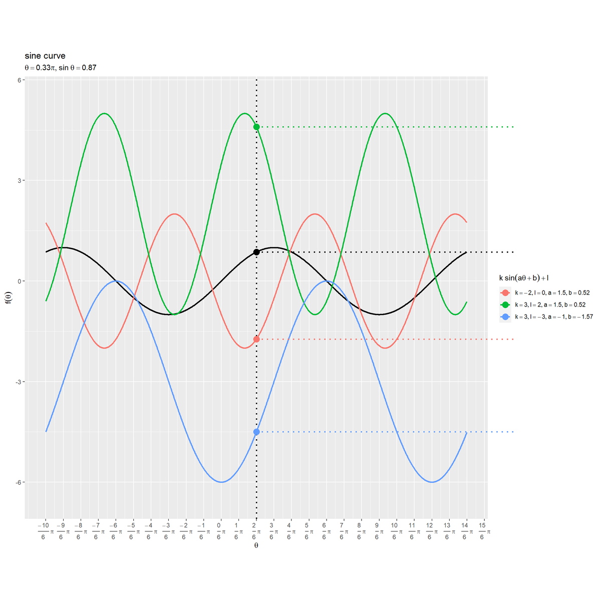
角度$\theta$を固定した$k \sin(a \theta + b) + l$をグラフで確認します。
パラメータと角度を指定します。
# パラメータを指定
k_i <- c(-2, 3, 3)
l_i <- c(0, 2, -3)
a_i <- c(1.5, 1.5, -1)
b_i <- c(1/6*pi, 1/6*pi, -1/2*pi)

# 曲線の数を設定
n <- length(k_i)

# 角度を指定
alpha <- 60

# ラジアンに変換
theta <- alpha / 180 * pi
theta
## [1] 1.047198
パラメータ$k, l, a, b$と角度(ラジアン)$\theta$を指定します。
パラメータを、それぞれk_i, l_i, a_i, b_iとして、同じ数の値を指定します。また指定した数をnとします。
・コード(クリックで展開)
曲線上に関数の点を描画するためのデータフレームを作成します。
# 因子レベルの設定用のベクトルを作成
param_level <- paste0("list(k==", k_i, ", l==", l_i, ", a==", a_i, ", b==", round(b_i, 2), ")")

# 関数の点の描画用
point_df <- tibble::tibble(
  theta = theta,
  sin_theta = sin(theta * a_i + b_i) * k_i + l_i,
  cos_theta = cos(theta * a_i + b_i) * k_i,
  param = paste0("list(k==", k_i, ", l==", l_i, ", a==", a_i, ", b==", round(b_i, 2), ")") |>
    factor(levels = param_level)
)
point_df
## # A tibble: 3 × 4
##   theta sin_theta cos_theta param
##   <dbl>     <dbl>     <dbl> <fct>
## 1  1.05     -1.73      1    list(k==-2, l==0, a==1.5, b==0.52)
## 2  1.05      4.60     -1.5  list(k==3, l==2, a==1.5, b==0.52)
## 3  1.05     -4.5      -2.60 list(k==3, l==-3, a==-1, b==-1.57)
$\theta$と$k \sin(a \theta + b) + l$、$k \cos(a \theta + b)$を格納します。
作図時の色分けなど用に、元の関数とパラメータによって加工した値を区別するための列paramを作成します。線の色付け順や凡例の表示順を設定する場合は、因子型にしてレベルを設定しておきます。
円を描画するためのデータフレームを作成します。
# 円の描画用
circle_df <- tidyr::expand_grid(
  i = 1:n, # 曲線番号
  theta = seq(from = 0, to = 2*pi, by = 0.05)
) |> # 曲線ごとに作図用のθを複製
  dplyr::group_by(i) |> # 角度の作成用
  dplyr::mutate(
    sin_theta = sin(theta) * k_i[unique(i)] + l_i[unique(i)],
    cos_theta = cos(theta) * k_i[unique(i)],
    param = paste0(
      "list(k==", k_i[unique(i)], ", l==", l_i[unique(i)],
      ", a==", a_i[unique(i)], ", b==", round(b_i[unique(i)], 2), ")"
    ) |>
    factor(levels = param_level)
  ) |>
  dplyr::ungroup()
circle_df
## # A tibble: 378 × 5
##        i theta sin_theta cos_theta param
##    <int> <dbl>     <dbl>     <dbl> <fct>
##  1     1  0        0         -2    list(k==-2, l==0, a==1.5, b==0.52)
##  2     1  0.05    -0.100     -2.00 list(k==-2, l==0, a==1.5, b==0.52)
##  3     1  0.1     -0.200     -1.99 list(k==-2, l==0, a==1.5, b==0.52)
##  4     1  0.15    -0.299     -1.98 list(k==-2, l==0, a==1.5, b==0.52)
##  5     1  0.2     -0.397     -1.96 list(k==-2, l==0, a==1.5, b==0.52)
##  6     1  0.25    -0.495     -1.94 list(k==-2, l==0, a==1.5, b==0.52)
##  7     1  0.3     -0.591     -1.91 list(k==-2, l==0, a==1.5, b==0.52)
##  8     1  0.35    -0.686     -1.88 list(k==-2, l==0, a==1.5, b==0.52)
##  9     1  0.4     -0.779     -1.84 list(k==-2, l==0, a==1.5, b==0.52)
## 10     1  0.45    -0.870     -1.80 list(k==-2, l==0, a==1.5, b==0.52)
## # … with 368 more rows
1からnの整数を曲線(パラメータの組み合わせ)番号として、円の作図用のラジアン$0 \leq \theta \leq 2 \pi$(theta列)との全ての組み合わせをexpand_grid()で作成します。これにより、パラメータの設定ごとにtheta列を複製できます。$a, b$の計算は、円周上を移動するだけなので、結果に影響しません。
i列でグループ化してパラメータの設定ごとに、$k \sin \theta + l$、$k \cos \theta$を計算します。
角度を表示するためのデータフレームを作成します。
# 半径の描画用
radius_df <- dplyr::bind_rows(
  tibble::tibble(
    x_from = 0,
    y_from = 0 + l_i,
    x_to = 1 * abs(k_i),
    y_to = 0 + l_i,
    param = paste0("list(k==", k_i, ", l==", l_i, ", a==", a_i, ", b==", round(b_i, 2), ")") |>
      factor(levels = param_level),
    k = k_i,
    type = "main"
  ), # 水平方向の半径
  tibble::tibble(
    x_from = 0,
    y_from = 0 + l_i,
    x_to = cos(theta * a_i + b_i) * k_i,
    y_to = sin(theta * a_i + b_i) * k_i + l_i,
    param = paste0("list(k==", k_i, ", l==", l_i, ", a==", a_i, ", b==", round(b_i, 2), ")") |>
      factor(levels = param_level),
    k = k_i,
    type = "main"
  ), # 角度aθ+bの半径
  tibble::tibble(
    x_from = 0,
    y_from = 0 + l_i,
    x_to = cos(theta * a_i + b_i) * abs(k_i),
    y_to = sin(theta * a_i + b_i) * abs(k_i) + l_i,
    param = paste0("list(k==", k_i, ", l==", l_i, ", a==", a_i, ", b==", round(b_i, 2), ")") |>
      factor(levels = param_level),
    k = k_i,
    type = "sub"
  ) # kが負のとき用の半径
) |>
  dplyr::group_by(k) |> # 行の抽出用
  dplyr::filter(
    (type == "main") | (k < 0 & type == "sub")
  ) |> # 不要な行を除去
  dplyr::ungroup()

# 角度マークの描画用
d <- 0.1
angle_df <- tibble::tibble(
  i = 1:n # 曲線番号
) |>
  dplyr::group_by(i) |> # 角度の作成用
  dplyr::summarise(
    theta = seq(from = min(0, theta*a_i[i]+b_i[i]), to = max(0, theta*a_i[i]+b_i[i]), length.out = 100),
    .groups = "keep"
  ) |>
  dplyr::mutate(
    x = cos(theta) * (unique(i)+1)*d,
    y = sin(theta) * (unique(i)+1)*d + l_i[unique(i)],
    param = paste0(
      "list(k==", k_i[unique(i)], ", l==", l_i[unique(i)],
      ", a==", a_i[unique(i)], ", b==", round(b_i, 2)[unique(i)], ")"
    ) |>
    factor(levels = param_level)
  ) |>
  dplyr::ungroup()

# 角度ラベルの描画用
angle_label_df <- angle_df |>
  dplyr::group_by(i, param) |> # 中点の計算用
  dplyr::summarise(
    theta = median(theta), .groups = "keep"
  ) |>
  dplyr::mutate(
    x = cos(theta) * (i+2)*d,
    y = sin(theta) * (i+2)*d + l_i[i],
    angle_label = paste0("theta[", i, "]")
  ) |>
  dplyr::ungroup()
radius_df; angle_df; angle_label_df
## # A tibble: 7 × 7
##   x_from y_from  x_to  y_to param                                  k type
##    <dbl>  <dbl> <dbl> <dbl> <fct>                              <dbl> <chr>
## 1      0      0  2     0    list(k==-2, l==0, a==1.5, b==0.52)    -2 main
## 2      0      2  3     2    list(k==3, l==2, a==1.5, b==0.52)      3 main
## 3      0     -3  3    -3    list(k==3, l==-3, a==-1, b==-1.57)     3 main
## 4      0      0  1    -1.73 list(k==-2, l==0, a==1.5, b==0.52)    -2 main
## 5      0      2 -1.5   4.60 list(k==3, l==2, a==1.5, b==0.52)      3 main
## 6      0     -3 -2.60 -4.5  list(k==3, l==-3, a==-1, b==-1.57)     3 main
## 7      0      0 -1     1.73 list(k==-2, l==0, a==1.5, b==0.52)    -2 sub
## # A tibble: 300 × 5
##        i  theta     x       y param
##    <int>  <dbl> <dbl>   <dbl> <fct>
##  1     1 0      0.2   0       list(k==-2, l==0, a==1.5, b==0.52)
##  2     1 0.0212 0.200 0.00423 list(k==-2, l==0, a==1.5, b==0.52)
##  3     1 0.0423 0.200 0.00846 list(k==-2, l==0, a==1.5, b==0.52)
##  4     1 0.0635 0.200 0.0127  list(k==-2, l==0, a==1.5, b==0.52)
##  5     1 0.0846 0.199 0.0169  list(k==-2, l==0, a==1.5, b==0.52)
##  6     1 0.106  0.199 0.0211  list(k==-2, l==0, a==1.5, b==0.52)
##  7     1 0.127  0.198 0.0253  list(k==-2, l==0, a==1.5, b==0.52)
##  8     1 0.148  0.198 0.0295  list(k==-2, l==0, a==1.5, b==0.52)
##  9     1 0.169  0.197 0.0337  list(k==-2, l==0, a==1.5, b==0.52)
## 10     1 0.190  0.196 0.0379  list(k==-2, l==0, a==1.5, b==0.52)
## # … with 290 more rows
## # A tibble: 3 × 6
##       i param                              theta     x      y angle_label
##   <int> <fct>                              <dbl> <dbl>  <dbl> <chr>
## 1     1 list(k==-2, l==0, a==1.5, b==0.52)  1.05 0.15   0.260 theta[1]
## 2     2 list(k==3, l==2, a==1.5, b==0.52)   1.05 0.2    2.35  theta[2]
## 3     3 list(k==3, l==-3, a==-1, b==-1.57) -1.31 0.129 -3.48  theta[3]
$0^{\circ}$と各$a \theta + b$における半径を描画するために、原点と円上の点を結ぶ線分の座標を格納してradius_dfとします。ただし、$k$が負の値の場合は、その角度$a \theta + b$の線分を破線で、反転させた線分を実線で描画することにします。
そこで、それぞれデータフレームに値を格納しておいてbind_rows()で結合し、filter()で不要な行($k$が正の値の場合の行)を取り除きます(もっと上手く処理できれば教えて下さい)。
各角度に応じた扇形(角度マーク)を描画するための値(ラジアン)を作成して、x軸とy軸の値を計算してangle_dfとします。
i列でグループ化して角ごとに、$0$から$a \theta + b$の値をsummarise()で作成します。
角度の中点に配置するように座標とラベル用の文字列を格納してangle_label_dfとします。
単位円におけるsin関数の値を描画するためのデータフレームを作成します。
# sin関数の線の描画用
sin_line_df <- tibble::tibble(
  i = 1:n, # 曲線番号
  x_from = cos(theta * a_i + b_i) * k_i,
  y_from = 0 + l_i,
  x_to = cos(theta * a_i + b_i) * k_i,
  y_to = sin(theta * a_i + b_i) * k_i + l_i,
  param = paste0("list(k==", k_i, ", l==", l_i, ", a==", a_i, ", b==", round(b_i, 2), ")") |>
    factor(levels = param_level)
)

# sin関数の線ラベルの描画用
sin_label_df <- sin_line_df |>
  dplyr::group_by(i) |> # 中点の計算用
  dplyr::mutate(
    # 中点に配置
    x = median(c(x_from, x_to)),
    y = median(c(y_from, y_to)),
    sin_theta = sin(theta * a_i[i] + b_i[i]) * k_i[i] + l_i[i],
    fnc_label = paste0("sin[", i, "]==", round(sin_theta, digits = 2))
  ) |>
  dplyr::ungroup() |>
  dplyr::select(x, y, param, fnc_label)
sin_line_df; sin_label_df
## # A tibble: 3 × 6
##       i x_from y_from  x_to  y_to param
##   <int>  <dbl>  <dbl> <dbl> <dbl> <fct>
## 1     1   1         0  1    -1.73 list(k==-2, l==0, a==1.5, b==0.52)
## 2     2  -1.5       2 -1.5   4.60 list(k==3, l==2, a==1.5, b==0.52)
## 3     3  -2.60     -3 -2.60 -4.5  list(k==3, l==-3, a==-1, b==-1.57)
## # A tibble: 3 × 4
##       x      y param                              fnc_label
##   <dbl>  <dbl> <fct>                              <chr>
## 1  1    -0.866 list(k==-2, l==0, a==1.5, b==0.52) sin[1]==-1.73
## 2 -1.5   3.30  list(k==3, l==2, a==1.5, b==0.52)  sin[2]==4.6
## 3 -2.60 -3.75  list(k==3, l==-3, a==-1, b==-1.57) sin[3]==-4.5
これまでと同様に処理します。
描画範囲を固定するための値を作成します。
# 描画領域のサイズを設定
d <- 0.5
x_min <- -max(abs(k_i)) - d
x_max <- max(abs(k_i)) + d
y_min <- -max(abs(k_i)) + min(l_i) - d
y_max <- max(abs(k_i)) + max(l_i) + d
l     <- 1.5
x_min; x_max; y_min; y_max
## [1] -3.5
## [1] 3.5
## [1] -6.5
## [1] 5.5
2つのグラフの描画範囲を固定するために、x軸の範囲をx_min, x_max、y軸の範囲をy_min, y_maxとして、また隣のグラフに届かないような長さlを指定します。
円上の点とsin関数上の点を結ぶ線(の半分)を描画するためのデータフレームを作成します。
# サイン波との対応用
segment_circle_df <- tibble::tibble(
  x_from = cos(theta * a_i + b_i) * k_i,
  y_from = sin(theta * a_i + b_i) * k_i + l_i,
  x_to = x_min-l,
  y_to = sin(theta * a_i + b_i) * k_i + l_i,
  param = paste0("list(k==", k_i, ", l==", l_i, ", a==", a_i, ", b==", round(b_i, 2), ")") |>
    factor(levels = param_level)
)
segment_circle_df
## # A tibble: 3 × 5
##   x_from y_from  x_to  y_to param
##    <dbl>  <dbl> <dbl> <dbl> <fct>
## 1   1     -1.73    -5 -1.73 list(k==-2, l==0, a==1.5, b==0.52)
## 2  -1.5    4.60    -5  4.60 list(k==3, l==2, a==1.5, b==0.52)
## 3  -2.60  -4.5     -5 -4.5  list(k==3, l==-3, a==-1, b==-1.57)
円周上の点からy軸への垂線を引くように座標を指定します。
ここまでは、設定したパラメータそれぞれに応じた値を持つ作図用のデータフレームを作成しました。
目安として表示するために、単位円における作図用のデータフレームを作成します。
# 単位円の描画用
unit_circle_df <- tibble::tibble(
  theta = seq(from = 0, to = 2*pi, by = 0.05),
  sin_theta = sin(theta),
  cos_theta = cos(theta)
)

# 角度目盛の描画用
tick_df <- tibble::tibble(
  alpha = 0:11 * 30,
  theta = 0:11 / 6 * pi,
  x = cos(theta),
  y = sin(theta),
  rad_label = paste0("frac(", 0:11, ", 6)~pi")
)

# 半径の描画用
unit_radius_df <- tibble::tibble(
  x_from = c(0, 0),
  y_from = c(0, 0),
  x_to = c(1, cos(theta)),
  y_to = c(0, sin(theta))
)

# 角度マークの描画用
d <- 0.1
unit_angle_df <- tibble::tibble(
  theta = seq(from = min(0, theta), to = max(0, theta), by = 0.1),
  x = cos(theta) * d,
  y = sin(theta) * d
)

# 角度ラベルの描画用
d <- 0.2
unit_angle_label_df <- tibble::tibble(
  theta = 0.5 * theta,
  x = cos(theta) * d,
  y = sin(theta) * d,
  angle_label = "theta"
)

# サイン波との対応用
segment_unit_circle_df <- tibble::tibble(
  x = cos(theta),
  y = sin(theta),
  x_to = x_min-l,
  y_to = sin(theta)
)
「sin関数の可視化」と同様の処理です。
単位円のグラフを作成します。
# 関数ラベルを作成
fnc_label <- paste0(
  "list(",
  "theta==", round(theta/pi, digits = 2), "*pi",
  ", sin~theta==", round(sin(theta), digits = 2),
  ", cos~theta==", round(cos(theta), digits = 2),
  ")"
)

# 円を作図
d <- 1.2
circle_graph <- ggplot() +
  geom_path(data = unit_circle_df,
            mapping = aes(x = cos_theta, y = sin_theta),
            size = 1) + # 単位円
  geom_text(data = tick_df,
            mapping = aes(x = x, y = y, angle = alpha+90),
            label = "|", size = 2) + # 角度目盛
  geom_text(data = tick_df,
            mapping = aes(x = x*d, y = y*d, label = rad_label,
                          hjust = 1-(x*0.5+0.5), vjust = 1-(y*0.5+0.5)), parse = TRUE) + # 角度目盛ラベル
  geom_segment(data = unit_radius_df,
               mapping = aes(x = x_from, y = y_from, xend = x_to, yend = y_to)) + # 角度θの半径
  geom_path(data = unit_angle_df,
            mapping = aes(x = x, y = y)) + # 角度θのマーク
  geom_text(data = unit_angle_label_df,
            mapping = aes(x = x, y = y, label = angle_label), parse = TRUE) + # 角度θのラベル
  geom_path(data = circle_df,
            mapping = aes(x = cos_theta, y = sin_theta, color = param),
            linetype = "dotted", size = 1) + # 半径kの円
  geom_segment(data = radius_df,
               mapping = aes(x = x_from, y = y_from, xend = x_to, yend = y_to,
                             color = param, linetype = type)) + # 角度aθ+bの半径
  geom_path(data = angle_df,
            mapping = aes(x = x, y = y, color = param)) + # 角度aθ+bのマーク
  geom_text(data = angle_label_df,
            mapping = aes(x = x, y = y, label = angle_label, color = param), parse = TRUE) + # 角度aθ+bのラベル
  geom_segment(data = sin_line_df,
               mapping = aes(x = x_from, y = y_from, xend = x_to, yend = y_to, color = param),
               size = 1) + # 角度aθ+bのsin関数
  geom_text(data = sin_label_df,
            mapping = aes(x = x, y = y, label = fnc_label, color = param), parse = TRUE,
            angle = 90, vjust = 1) + # 角度aθ+bのsin関数ラベル
  geom_segment(data = segment_unit_circle_df,
               mapping = aes(x = x, y = y, xend = x_to, yend = y_to),
               size = 1, linetype = "dotted") + # 角度θのsin波との対応線
  geom_point(data = segment_unit_circle_df,
             mapping = aes(x = x, y = y),
             size = 4) + # 角度θの点
  geom_segment(data = segment_circle_df,
               mapping = aes(x = x_from, y = y_from, xend = x_to, yend = y_to, color = param),
               size = 1, linetype = "dotted") + # 角度aθ+bのsin波との対応線
  geom_point(data = point_df,
             mapping = aes(x = cos_theta, y = sin_theta, color = param),
             size = 4) + # 円上の点
  scale_linetype_manual(breaks = c("main", "sub"),
                        values = c("solid", "dashed")) + # 線の種類
  scale_color_hue(breaks = point_df[["param"]],
                  labels = parse(text = as.character(point_df[["param"]])),
                  name = expression(k~sin(a*theta+b)+l)) + # 線の色の凡例
  theme(legend.position = "none") + # 凡例の非表示
  coord_fixed(ratio = 1, clip = "off",
              xlim = c(x_min, x_max), ylim = c(y_min, y_max)) + # 描画領域
  labs(title = "unit circle",
       subtitle = parse(text = fnc_label),
       x = "x", y = "y")
circle_graph

これまでと同様に、単位円$(\cos(\theta), \sin(\theta))$とパラメータごとの円$(k \cos(\theta) + l, k \sin(\theta) + l)$に関して作図します。
サイン波の作図用のラジアンの値を作成します。
# 作図用のラジアンの値を作成
theta_vals <- seq(from = theta-2*pi, to = theta+2*pi, by = 0.01)
この例では、2周期分の値を指定します。
サイン波の描画するためのデータフレームを作成します。
# サイン波の描画用
sin_curve_df <- tidyr::expand_grid(
  i = 1:n, # 曲線番号
  theta = theta_vals
) |> # 曲線ごとに作図用のθを複製
  dplyr::group_by(i) |>
  dplyr::mutate(
    sin_theta = sin(theta * a_i[unique(i)] + b_i[unique(i)]) * k_i[unique(i)] + l_i[unique(i)],
    param = paste0(
      "list(k==", k_i[unique(i)], ", l==", l_i[unique(i)],
      ", a==", a_i[unique(i)], ", b==", round(b_i[unique(i)], 2), ")"
    ) |>
      factor(levels = param_level)
  ) |>
  dplyr::ungroup()
sin_curve_df
## # A tibble: 3,771 × 4
##        i theta sin_theta param
##    <int> <dbl>     <dbl> <fct>
##  1     1 -5.24      1.73 list(k==-2, l==0, a==1.5, b==0.52)
##  2     1 -5.23      1.72 list(k==-2, l==0, a==1.5, b==0.52)
##  3     1 -5.22      1.70 list(k==-2, l==0, a==1.5, b==0.52)
##  4     1 -5.21      1.69 list(k==-2, l==0, a==1.5, b==0.52)
##  5     1 -5.20      1.67 list(k==-2, l==0, a==1.5, b==0.52)
##  6     1 -5.19      1.65 list(k==-2, l==0, a==1.5, b==0.52)
##  7     1 -5.18      1.64 list(k==-2, l==0, a==1.5, b==0.52)
##  8     1 -5.17      1.62 list(k==-2, l==0, a==1.5, b==0.52)
##  9     1 -5.16      1.60 list(k==-2, l==0, a==1.5, b==0.52)
## 10     1 -5.15      1.58 list(k==-2, l==0, a==1.5, b==0.52)
## # … with 3,761 more rows
作図用の値theta_valsをexpand_grid()で複製して、$\theta$と$k \sin(a \theta + b) + l$を計算します。
先ほどと同様に、sin関数上の点と円周上の点を結ぶ線(の半分)を描画するためのデータフレームを作成します。
# x軸(角度)・円との対応用
d <- 1.1
segment_sin_df <- tibble::tibble(
  x_from = theta,
  y_from = sin(theta * a_i + b_i) * k_i + l_i,
  x_to = max(theta_vals)+l,
  y_to = sin(theta * a_i + b_i) * k_i + l_i,
  param = paste0("list(k==", k_i, ", l==", l_i, ", a==", a_i, ", b==", round(b_i, 2), ")") |>
    factor(levels = param_level)
)
segment_sin_df
## # A tibble: 3 × 5
##   x_from y_from  x_to  y_to param
##    <dbl>  <dbl> <dbl> <dbl> <fct>
## 1   1.05  -1.73  8.82 -1.73 list(k==-2, l==0, a==1.5, b==0.52)
## 2   1.05   4.60  8.82  4.60 list(k==3, l==2, a==1.5, b==0.52)
## 3   1.05  -4.5   8.82 -4.5  list(k==3, l==-3, a==-1, b==-1.57)
曲線上の点からx軸・y軸への垂線を引くように座標を指定します。
また、元のsin関数と単位円上の点を結ぶ線(の半分)を描画するためのデータフレームを作成します。
# サイン波の描画用
unit_sin_curve_df <- tibble::tibble(
  theta = theta_vals,
  sin_theta = sin(theta_vals)
)

# x軸(角度)・単位円との対応用
segment_unit_sin_df <- tibble::tibble(
  x = theta,
  y = sin(theta) ,
  x_to = max(theta_vals)+l,
  y_to = sin(theta)
)
曲線上の点からy軸への垂線を引くように座標を指定します。x, y列は、曲線上の点などを描画するのにも使います。
x軸目盛として、角度ラベルを描画するのに用いるベクトルを作成します。
# x軸目盛ラベルの描画用の値を作成
tick_min <- floor(min(theta_vals) * 6 / pi)
tick_vec <- seq(from = tick_min, to = tick_min+25, by = 1)
「関数をk倍する場合」と同じ処理です。
サイン波のグラフを作成します。
# 関数ラベルを作成
fnc_label <- paste0(
  "list(",
  "theta==", round(theta/pi, digits = 2), "*pi",
  ", sin~theta==", round(sin(theta), digits = 2),
  ")"
)

# サイン波を作図
sin_graph <- ggplot() +
  geom_line(data = unit_sin_curve_df,
            mapping = aes(x = theta, y = sin_theta),
            size = 1) + # 角度θのsin関数
  geom_segment(data = segment_unit_sin_df,
               mapping = aes(x = x, y = y, xend = x_to, yend = y_to),
               size = 1, linetype = "dotted") + # 角度θの単位円との対応線
  geom_vline(data = segment_unit_sin_df,
             mapping = aes(xintercept = x),
             size = 1, linetype = "dotted") + # 角度θの単位円との対応線
  geom_point(data = segment_unit_sin_df,
             mapping = aes(x = x, y = y),
             size = 4) + # 角度θの関数曲線上の点
  geom_line(data = sin_curve_df,
            mapping = aes(x = theta, y = sin_theta, color = param),
            size = 1) + # 角度aθ+bのsin関数
  geom_segment(data = segment_sin_df,
               mapping = aes(x = x_from, y = y_from, xend = x_to, yend = y_to, color = param),
               size = 1, linetype = "dotted") + # 角度aθ+bの円との対応線
  geom_point(data = point_df,
             mapping = aes(x = theta, y = sin_theta, color = param),
             size = 4) + # 角度aθ+bの関数曲線上の点
  scale_x_continuous(breaks = tick_vec/6*pi,
                     labels = parse(text = paste0("frac(", tick_vec, ", 6)~pi"))) + # 角度目盛ラベル
  scale_color_hue(breaks = point_df[["param"]],
                  labels = parse(text = as.character(point_df[["param"]])),
                  name = expression(k~sin(a*theta+b)+l)) +
  theme(legend.text.align = 0) + # 凡例の左揃え
  coord_fixed(ratio = 1, clip = "off",
              xlim = c(min(theta_vals), max(theta_vals)), ylim = c(y_min, y_max)) + # 描画領域
  labs(title = "sine curve",
       subtitle = parse(text = fnc_label),
       x = expression(theta), y = expression(f(theta)))
sin_graph
これまでと同様に、元のsin関数$\sin \theta$とパラメータごとのsin関数$k \sin(a \theta + b) + l$に関して作図します。
2つのグラフを並べて描画します。
# グラフを並べて描画
patchwork::wrap_plots(sin_graph, circle_graph) +
  patchwork::plot_layout(guides = "collect")

$l$の値によってグラフ全体がy軸方向に変化するのを確認できます。
アニメーションの作成
続いて、角度を変化させたアニメーションで確認します。
フレーム数とパラメータ、角度の範囲を指定して、角度として用いる値を作成します。
# フレーム数を指定
frame_num <- 100

# パラメータを指定
k_i <- c(-2, 3, 3)
l_i <- c(0, 2, -3)
a_i <- c(1.5, 1.5, -1)
b_i <- c(1/6*pi, 1/6*pi, -1/2*pi)

# 曲線の数を設定
n <- length(k_i)

# 角度の範囲を指定
theta_min <- -2 * pi
theta_max <- 2 * pi

# フレームごとの角度を作成
theta_i <- seq(from = theta_min, to = theta_max, length.out = frame_num+1)[1:frame_num]
「関数をk倍する場合」と同じ処理です。
・コード(クリックで展開)
theta_iから順番に値を取り出して作図し、グラフを書き出します
# 一時保存フォルダを指定
dir_path <- "tmp_folder"

# 描画領域のサイズを設定
d <- 0.5
x_min <- -max(abs(k_i)) - d
x_max <- max(abs(k_i)) + d
y_min <- -max(abs(k_i)) + min(l_i) - d
y_max <- max(abs(k_i)) + max(l_i) + d
l     <- 1.5

# 円の描画用
circle_df <- tidyr::expand_grid(
  i = 1:n, # 曲線番号
  theta = seq(from = 0, to = 2*pi, by = 0.05)
) |> # 曲線ごとに作図用のθを複製
  dplyr::group_by(i) |> # 角度の作成用
  dplyr::mutate(
    sin_theta = sin(theta) * k_i[unique(i)] + l_i[unique(i)],
    cos_theta = cos(theta) * k_i[unique(i)],
    param = paste0(
      "list(k==", k_i[unique(i)], ", l==", l_i[unique(i)],
      ", a==", a_i[unique(i)], ", b==", round(b_i[unique(i)], 2), ")"
    ) |>
    factor(levels = param_level)
  ) |>
  dplyr::ungroup()

# 角度ごとに作図
for(i in 1:frame_num) {

  # i番目の角度を取得
  theta <- theta_i[i]

  # 因子レベルの設定用のベクトルを作成
  param_level <- paste0("list(k==", k_i, ", l==", l_i, ", a==", a_i, ", b==", round(b_i, 2), ")")

  # 関数の点の描画用
  point_df <- tibble::tibble(
    theta = theta,
    sin_theta = sin(theta * a_i + b_i) * k_i + l_i,
    cos_theta = cos(theta * a_i + b_i) * k_i,
    param = paste0("list(k==", k_i, ", l==", l_i, ", a==", a_i, ", b==", round(b_i, 2), ")") |>
      factor(levels = param_level)
  )

  # 半径の描画用
  radius_df <- dplyr::bind_rows(
    tibble::tibble(
      x_from = 0,
      y_from = 0 + l_i,
      x_to = 1 * abs(k_i),
      y_to = 0 + l_i,
      param = paste0("list(k==", k_i, ", l==", l_i, ", a==", a_i, ", b==", round(b_i, 2), ")") |>
        factor(levels = param_level),
      k = k_i,
      type = "main"
    ), # 水平方向の半径
    tibble::tibble(
      x_from = 0,
      y_from = 0 + l_i,
      x_to = cos(theta * a_i + b_i) * k_i,
      y_to = sin(theta * a_i + b_i) * k_i + l_i,
      param = paste0("list(k==", k_i, ", l==", l_i, ", a==", a_i, ", b==", round(b_i, 2), ")") |>
        factor(levels = param_level),
      k = k_i,
      type = "main"
    ), # 角度aθ+bの半径
    tibble::tibble(
      x_from = 0,
      y_from = 0 + l_i,
      x_to = cos(theta * a_i + b_i) * abs(k_i),
      y_to = sin(theta * a_i + b_i) * abs(k_i) + l_i,
      param = paste0("list(k==", k_i, ", l==", l_i, ", a==", a_i, ", b==", round(b_i, 2), ")") |>
        factor(levels = param_level),
      k = k_i,
      type = "sub"
    ) # kが負のとき用の半径
  ) |>
    dplyr::group_by(k) |> # 行の抽出用
    dplyr::filter(
      (type == "main") | (k < 0 & type == "sub")
    ) |> # 不要な行を除去
    dplyr::ungroup()

  # 角度マークの描画用
  d <- 0.1
  angle_df <- tibble::tibble(
    i = 1:n # 曲線番号
  ) |>
    dplyr::group_by(i) |> # 角度の作成用
    dplyr::summarise(
      theta = seq(from = min(0, theta*a_i[i]+b_i[i]), to = max(0, theta*a_i[i]+b_i[i]), length.out = 100),
      .groups = "keep"
    ) |>
    dplyr::mutate(
      x = cos(theta) * (unique(i)+1)*d,
      y = sin(theta) * (unique(i)+1)*d + l_i[unique(i)],
      param = paste0(
        "list(k==", k_i[unique(i)], ", l==", l_i[unique(i)],
        ", a==", a_i[unique(i)], ", b==", round(b_i, 2)[unique(i)], ")"
      ) |>
      factor(levels = param_level)
    ) |>
    dplyr::ungroup()

  # 角度ラベルの描画用
  angle_label_df <- angle_df |>
    dplyr::group_by(i, param) |> # 中点の計算用
    dplyr::summarise(
      theta = median(theta), .groups = "keep"
    ) |>
    dplyr::mutate(
      x = cos(theta) * (i+2)*d,
      y = sin(theta) * (i+2)*d + l_i[i],
      angle_label = paste0("theta[", i, "]")
    ) |>
    dplyr::ungroup()

  # sin関数の線の描画用
  sin_line_df <- tibble::tibble(
    i = 1:n, # 曲線番号
    x_from = cos(theta * a_i + b_i) * k_i,
    y_from = 0 + l_i,
    x_to = cos(theta * a_i + b_i) * k_i,
    y_to = sin(theta * a_i + b_i) * k_i + l_i,
    param = paste0("list(k==", k_i, ", l==", l_i, ", a==", a_i, ", b==", round(b_i, 2), ")") |>
      factor(levels = param_level)
  )

  # sin関数の線ラベルの描画用
  sin_label_df <- sin_line_df |>
    dplyr::group_by(i) |> # 中点の計算用
    dplyr::mutate(
      # 中点に配置
      x = median(c(x_from, x_to)),
      y = median(c(y_from, y_to)),
      sin_theta = sin(theta * a_i[i] + b_i[i]) * k_i[i] + l_i[i],
      fnc_label = paste0("sin[", i, "]==", round(sin_theta, digits = 2))
    ) |>
    dplyr::ungroup() |>
    dplyr::select(x, y, param, fnc_label)

  # サイン波との対応用
  segment_circle_df <- tibble::tibble(
    x_from = cos(theta * a_i + b_i) * k_i,
    y_from = sin(theta * a_i + b_i) * k_i + l_i,
    x_to = x_min-l,
    y_to = sin(theta * a_i + b_i) * k_i + l_i,
    param = paste0("list(k==", k_i, ", l==", l_i, ", a==", a_i, ", b==", round(b_i, 2), ")") |>
      factor(levels = param_level)
  )

  # 半径の描画用
  unit_radius_df <- tibble::tibble(
    x_from = c(0, 0),
    y_from = c(0, 0),
    x_to = c(1, cos(theta)),
    y_to = c(0, sin(theta))
  )

  # 角度マークの描画用
  d <- 0.1
  unit_angle_df <- tibble::tibble(
    theta = seq(from = min(0, theta), to = max(0, theta), by = 0.1),
    x = cos(theta) * d,
    y = sin(theta) * d
  )

  # 角度ラベルの描画用
  d <- 0.2
  unit_angle_label_df <- tibble::tibble(
    theta = 0.5 * theta,
    x = cos(theta) * d,
    y = sin(theta) * d,
    angle_label = "theta"
  )

  # サイン波との対応用
  segment_unit_circle_df <- tibble::tibble(
    x = cos(theta),
    y = sin(theta),
    x_to = x_min-l,
    y_to = sin(theta)
  )

  # 関数ラベルを作成
  fnc_label <- paste0(
    "list(",
    "theta==", round(theta/pi, digits = 2), "*pi",
    ", sin~theta==", round(sin(theta), digits = 2),
    ", cos~theta==", round(cos(theta), digits = 2),
    ")"
  )

  # 円を作図
  d <- 1.2
  circle_graph <- ggplot() +
    geom_path(data = unit_circle_df,
              mapping = aes(x = cos_theta, y = sin_theta),
              size = 1) + # 単位円
    geom_text(data = tick_df,
              mapping = aes(x = x, y = y, angle = alpha+90),
              label = "|", size = 2) + # 角度目盛
    geom_text(data = tick_df,
              mapping = aes(x = x*d, y = y*d, label = rad_label,
                            hjust = 1-(x*0.5+0.5), vjust = 1-(y*0.5+0.5)), parse = TRUE) + # 角度目盛ラベル
    geom_segment(data = unit_radius_df,
                 mapping = aes(x = x_from, y = y_from, xend = x_to, yend = y_to)) + # 角度θの半径
    geom_path(data = unit_angle_df,
              mapping = aes(x = x, y = y)) + # 角度θのマーク
    geom_text(data = unit_angle_label_df,
              mapping = aes(x = x, y = y, label = angle_label), parse = TRUE) + # 角度θのラベル
    geom_path(data = circle_df,
              mapping = aes(x = cos_theta, y = sin_theta, color = param),
              linetype = "dotted", size = 1) + # 半径kの円
    geom_segment(data = radius_df,
                 mapping = aes(x = x_from, y = y_from, xend = x_to, yend = y_to,
                               color = param, linetype = type)) + # 角度aθ+bの半径
    geom_path(data = angle_df,
              mapping = aes(x = x, y = y, color = param)) + # 角度aθ+bのマーク
    geom_text(data = angle_label_df,
              mapping = aes(x = x, y = y, label = angle_label, color = param), parse = TRUE) + # 角度aθ+bのラベル
    geom_segment(data = sin_line_df,
                 mapping = aes(x = x_from, y = y_from, xend = x_to, yend = y_to, color = param),
                 size = 1) + # 角度aθ+bのsin関数
    geom_text(data = sin_label_df,
              mapping = aes(x = x, y = y, label = fnc_label, color = param), parse = TRUE,
              angle = 90, vjust = 1) + # 角度aθ+bのsin関数ラベル
    geom_segment(data = segment_unit_circle_df,
                 mapping = aes(x = x, y = y, xend = x_to, yend = y_to),
                 linetype = "dotted") + # 角度θのsin波との対応線
    geom_point(data = segment_unit_circle_df,
               mapping = aes(x = x, y = y),
               size = 4) + # 角度θの点
    geom_segment(data = segment_circle_df,
                 mapping = aes(x = x_from, y = y_from, xend = x_to, yend = y_to, color = param),
                 linetype = "dotted") + # 角度aθ+bのsin波との対応線
    geom_point(data = point_df,
               mapping = aes(x = cos_theta, y = sin_theta, color = param),
               size = 4) + # 円上の点
    scale_linetype_manual(breaks = c("main", "sub"),
                          values = c("solid", "dashed")) + # 線の種類
    scale_color_hue(breaks = point_df[["param"]],
                    labels = parse(text = as.character(point_df[["param"]])),
                    name = expression(k~sin(a*theta+b)+l)) + # 線の色の凡例
    theme(legend.position = "none") + # 凡例の非表示
    coord_fixed(ratio = 1, clip = "off",
                xlim = c(x_min, x_max), ylim = c(y_min, y_max)) + # 描画領域
    labs(title = "unit circle",
         subtitle = parse(text = fnc_label),
         x = "x", y = "y")

  # 作図用のラジアンの値を作成
  theta_size <- 2 * pi
  theta_vals <- seq(from = max(theta_min, theta-theta_size), to = theta, by = 0.01)

  # サイン波の描画用
  sin_curve_df <- tidyr::expand_grid(
    i = 1:n, # 曲線番号
    theta = theta_vals
  ) |> # 曲線ごとに作図用のθを複製
    dplyr::group_by(i) |>
    dplyr::mutate(
      sin_theta = sin(theta * a_i[unique(i)] + b_i[unique(i)]) * k_i[unique(i)] + l_i[unique(i)],
      param = paste0(
        "list(k==", k_i[unique(i)], ", l==", l_i[unique(i)],
        ", a==", a_i[unique(i)], ", b==", round(b_i[unique(i)], 2), ")"
      ) |>
        factor(levels = param_level)
    ) |>
    dplyr::ungroup()

  # x軸(角度)・円との対応用
  d <- 1.1
  segment_sin_df <- tibble::tibble(
    x_from = theta,
    y_from = sin(theta * a_i + b_i) * k_i + l_i,
    x_to = max(theta_vals)+l,
    y_to = sin(theta * a_i + b_i) * k_i + l_i,
    param = paste0("list(k==", k_i, ", l==", l_i, ", a==", a_i, ", b==", round(b_i, 2), ")") |>
      factor(levels = param_level)
  )

  # サイン波の描画用
  unit_sin_curve_df <- tibble::tibble(
    theta = theta_vals,
    sin_theta = sin(theta_vals)
  )

  # x軸(角度)・単位円との対応用
  segment_unit_sin_df <- tibble::tibble(
    x = theta,
    y = sin(theta) ,
    x_to = max(theta_vals)+l,
    y_to = sin(theta)
  )

  # x軸目盛ラベルの描画用の値を作成
  tick_min <- floor((theta-theta_size) * 6 / pi)
  tick_vec <- seq(from = tick_min, to = tick_min+13, by = 1)

  # 関数ラベルを作成
  fnc_label <- paste0(
    "list(",
    "theta==", round(theta/pi, digits = 2), "*pi",
    ", sin~theta==", round(sin(theta), digits = 2),
    ")"
  )

  # サイン波を作図
  sin_graph <- ggplot() +
    geom_line(data = unit_sin_curve_df,
              mapping = aes(x = theta, y = sin_theta),
              size = 1) + # 角度θのsin関数
    geom_segment(data = segment_unit_sin_df,
                 mapping = aes(x = x, y = y, xend = x_to, yend = y_to),
                 linetype = "dotted") + # 角度θの単位円との対応線
    geom_vline(data = segment_unit_sin_df,
               mapping = aes(xintercept = x),
               linetype = "dotted") + # 角度θの単位円との対応線
    geom_point(data = segment_unit_sin_df,
               mapping = aes(x = x, y = y),
               size = 4) + # 角度θの関数曲線上の点
    geom_line(data = sin_curve_df,
              mapping = aes(x = theta, y = sin_theta, color = param),
              size = 1) + # 角度aθ+bのsin関数
    geom_segment(data = segment_sin_df,
                 mapping = aes(x = x_from, y = y_from, xend = x_to, yend = y_to, color = param),
                 linetype = "dotted") + # 角度aθ+bの円との対応線
    geom_point(data = point_df,
               mapping = aes(x = theta, y = sin_theta, color = param),
               size = 4) + # 角度aθ+bの関数曲線上の点
    scale_x_continuous(breaks = tick_vec/6*pi,
                       labels = parse(text = paste0("frac(", tick_vec, ", 6)~pi"))) + # 角度目盛ラベル
    scale_color_hue(breaks = point_df[["param"]],
                    labels = parse(text = as.character(point_df[["param"]])),
                    name = expression(k~sin(a*theta+b)+l)) +
    theme(legend.text.align = 0) + # 凡例の左揃え
    coord_fixed(ratio = 1, clip = "off",
                xlim = c(theta-theta_size, theta), ylim = c(y_min, y_max)) + # 描画領域
    labs(title = "sine curve",
         subtitle = parse(text = fnc_label),
         x = expression(theta), y = expression(f(theta)))

  # グラフを並べて描画
  graph <- patchwork::wrap_plots(sin_graph, circle_graph) +
      patchwork::plot_layout(guides = "collect")

  # ファイルを書き出し
  file_path <- paste0(dir_path, "/", stringr::str_pad(i, width = nchar(frame_num), pad = "0"), ".png")
  ggplot2::ggsave(filename = file_path, plot = graph, width = 1500, height = 1000, units = "px", dpi = 100)

  # 途中経過を表示
  message("\r", i, "/", frame_num, appendLF = FALSE)
}
「グラフの作成」で作成したunit_circle_df, tick_dfも使います。
「関数をk倍する場合」のコードでgif画像を作成します。
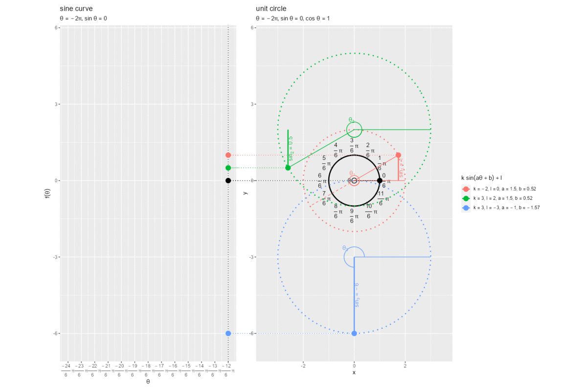
色々比較してみてください。
この記事では、sin関数の変形を確認しました。
おわりに
ほぼ初めて三角関数の勉強をしているのでへーとかおーとか言いながら書きました。
いくつか適切な用語が分からず書いてる部分があります。おかしければ指摘していただけると嬉しいです。
重複したコードが載りすぎてるだけなんですが、久しぶりに1記事で10万文字を超えました。別記事にしようか悩んだのですが、まとまってる方が分かりやすいよなと判断しました。作図コード目当てに読む人も少ないと思いますし、図を流し見しやすいように構成したつもりです。
先ほど公開された新曲のMVをどうぞ。
見蕩れてしまう。
【次の内容】
つづく