はじめに
『スタンフォード ベクトル・行列からはじめる最適化数学』の学習ノートです。
「数式の行間埋め」や「Pythonを使っての再現」によって理解を目指します。本と一緒に読んでください。
この記事は5.4節「グラム・シュミット法」の内容です。
グラム・シュミット法により正規直交ベクトルを作成します。
【前の内容】
【他の内容】
【今回の内容】
グラム・シュミット法の可視化
グラム・シュミット法(Gram-Schmidt algorithm)による正規直交ベクトル(orthonormal vector)の作成過程(ベクトルの正規直交化(orthogonalization)の過程)をグラフで確認します。
線形結合については「【Python】1.3:ベクトルの線形結合の可視化【『スタンフォード線形代数入門』のノート】 - からっぽのしょこ」、ノルムについては「【Python】3.1:ユークリッドノルムの可視化【『スタンフォード線形代数入門』のノート】 - からっぽのしょこ」を参照してください。
利用するライブラリを読み込みます。
# 利用ライブラリ
import numpy as np
import matplotlib.pyplot as plt
from matplotlib.animation import FuncAnimation
2次元の場合
まずは、2次元空間(平面)上でグラム・シュミット法によるベクトルの正規直交化(正規直交ベクトルの作成)を可視化します。
単位円を描画するための配列を作成しておきます。
# 単位円用のラジアンを作成
t_vals = np.linspace(start=0.0, stop=2.0*np.pi, num=201)
print(t_vals[:5])

# 単位円の座標を計算
x_vals = np.cos(t_vals)
y_vals = np.sin(t_vals)
print(np.linalg.norm(np.stack([x_vals.flatten(), y_vals.flatten()]), axis=0)[:5])
[0.         0.03141593 0.06283185 0.09424778 0.12566371]
[1. 1. 1. 1. 1.]
のラジアン(弧度法における角度)を作成して、単位円の座標
、
を計算します。
単位円は、原点からの距離(ノルム)が1の点(座標)を表します。
正規直交化の計算
正規直交化の計算(処理)を1つずつ確認します。
2次元ベクトルを指定します。
# ベクトルを指定
a1 = np.array([2.0, 3.0])
a2 = np.array([1.0, -2.0])
2つのベクトルを
a1, a2として値を指定します。ただし、線形独立(を満たす係数が
のときのみ)であり、どちらも0ベクトルでない(
である)必要があります。Pythonでは0からインデックスが割り当てられるので、
の値は
a1[0]に対応します。
2次元空間上に2つのベクトルを描画します。
# サイズ用の値を設定
x_min = np.floor(np.min([-1.0, a1[0], a2[0]])) - 1
x_max = np.ceil(np.max([1.0, a1[0], a2[0]])) + 1
y_min = np.floor(np.min([-1.0, a1[1], a2[1]])) - 1
y_max = np.ceil(np.max([1.0, a1[1], a2[1]])) + 1

# 元のベクトルを作図
fig, ax = plt.subplots(figsize=(6, 6), facecolor='white')
ax.plot(x_vals, y_vals, color='black') # 単位円
ax.quiver(0, 0, *a1,
          color='red', width=0.01, headwidth=5, headlength=5,
          angles='xy', scale_units='xy', scale=1,
          label='$a_1=('+', '.join(map(str, a1))+')$') # ベクトルa1
ax.quiver(0, 0, *a2,
          color='blue', width=0.01, headwidth=5, headlength=5,
          angles='xy', scale_units='xy', scale=1,
          label='$a_2=('+', '.join(map(str, a2))+')$') # ベクトルa2
ax.set_xticks(ticks=np.arange(x_min, x_max+1))
ax.set_yticks(ticks=np.arange(y_min, y_max+1))
ax.set_xlabel('$x_1$')
ax.set_ylabel('$x_2$')
ax.grid()
ax.set_title('$\\beta_1 a_1 + \\beta_2 a_2 \\neq 0\ (\\beta_1 \\neq \\beta_2 \\neq 0)$', fontsize=20)
ax.legend()
ax.set_aspect('equal')
plt.show()

axes.quiver()でベクトルを描画します。第1・2引数に始点の座標、第3・4引数にベクトルのサイズ(変化量)を指定します。その他に、指定した値の通りに(調整せずに)矢印を描画するための設定をしています。
配列a1, a2の前に*を付けてアンパック(展開)して指定しています。
1番目のベクトルを複製して
とします。
# 1番目のベクトルを複製(1番目の直交ベクトルを作成)
q1_tilde = a1.copy()
print(q1_tilde)
[2. 3.]
のベクトルを
q1_tildeとして作成します。
を描画します。
作図コード(クリックで展開)
# 1番目の直交ベクトルを作図
fig, ax = plt.subplots(figsize=(6, 6), facecolor='white')
ax.plot(x_vals, y_vals, color='black') # 単位円
ax.quiver(0, 0, *a1,
          fc='none', ec='red', ls=':', lw=1, width=0.001, headwidth=50, headlength=50,
          angles='xy', scale_units='xy', scale=1,
          label='$a_1=('+', '.join(map(str, a1))+')$') # ベクトルa1
ax.quiver(0, 0, *a2,
          color='blue', width=0.01, headwidth=5, headlength=5,
          angles='xy', scale_units='xy', scale=1) # ベクトルa2
ax.quiver(0, 0, *q1_tilde,
          color='red', width=0.01, headwidth=5, headlength=5,
          angles='xy', scale_units='xy', scale=1,
          label='$\\tilde{q}_1=('+', '.join(map(str, q1_tilde))+')$') # ベクトルq~1
ax.set_xticks(ticks=np.arange(x_min, x_max+1))
ax.set_yticks(ticks=np.arange(y_min, y_max+1))
ax.set_xlabel('$x_1$')
ax.set_ylabel('$x_2$')
ax.grid()
ax.set_title('$\\tilde{q}_1 = a_1$', fontsize=20)
ax.legend()
ax.set_aspect('equal')
plt.show()

と
は同じベクトルなので、重なって片方が見えていません。
を正規化して
とします。
# 1番目の直交ベクトルを正規化
norm_q1_tilde = np.linalg.norm(q1_tilde)
q1 = q1_tilde / norm_q1_tilde
print(q1)
print(np.linalg.norm(q1))
[0.5547002  0.83205029]
1.0
をユークリッドノルム
で割って正規化
します。ノルムは
np.linalg.norm()で計算できます。
正規化したベクトルはになります(ノルムを1にすることを正規化すると言います)。
を描画します。
作図コード(クリックで展開)
# 1番目の正規直交ベクトルを作図
fig, ax = plt.subplots(figsize=(6, 6), facecolor='white')
ax.plot(x_vals, y_vals, color='black') # 単位円
ax.quiver(0, 0, *a2,
          color='blue', width=0.01, headwidth=5, headlength=5,
          angles='xy', scale_units='xy', scale=1) # ベクトルa2
ax.quiver(0, 0, *q1_tilde,
          fc='none', ec='red', ls=':', lw=1, width=0.001, headwidth=50, headlength=50,
          angles='xy', scale_units='xy', scale=1,
          label='$\\tilde{q}_1=('+', '.join(map(str, q1_tilde))+')$') # ベクトルq~1
ax.quiver(0, 0, *q1,
          color='red', width=0.01, headwidth=5, headlength=5,
          angles='xy', scale_units='xy', scale=1,
          label='$q_1=('+', '.join(map(str, q1.round(1)))+')$') # ベクトルq1
ax.set_xticks(ticks=np.arange(x_min, x_max+1))
ax.set_yticks(ticks=np.arange(y_min, y_max+1))
ax.set_xlabel('$x_1$')
ax.set_ylabel('$x_2$')
ax.grid()
ax.set_title('$q_1 = \\frac{\\tilde{q}_1}{\|\\tilde{q}_1\|}$', fontsize=20)
ax.legend()
ax.set_aspect('equal')
plt.show()

が、
と同じ方向で、ノルムが1の(原点から単位円上の点への移動を表す)ベクトルなのが分かります。
の内積を係数として、
の線形結合を
とします。
# 2番目の直交ベクトルを計算
beta1 = np.dot(q1, a2)
q2_tilde = a2 - beta1 * q1
print(q2_tilde)
[ 1.61538462 -1.07692308]
を計算して
q2_tildeとします。内積はnp.dot()で計算できます。
を描画します。
作図コード(クリックで展開)
# 2番目の直交ベクトルを作図
fig, ax = plt.subplots(figsize=(6, 6), facecolor='white')
ax.plot(x_vals, y_vals, color='black') # 単位円
ax.quiver(0, 0, *a2,
          fc='none', ec='blue', ls=':', lw=1, width=0.001, headwidth=50, headlength=50,
          angles='xy', scale_units='xy', scale=1,
          label='$a_2=('+', '.join(map(str, a2))+')$') # ベクトルa2
ax.quiver(0, 0, *q1,
          color='red', width=0.01, headwidth=5, headlength=5,
          angles='xy', scale_units='xy', scale=1) # ベクトルq1
ax.quiver(*a2, *-beta1*q1,
          color='purple', width=0.01, headwidth=5, headlength=5,
          angles='xy', scale_units='xy', scale=1,
          label='$- (q_1^{\\top} a_2) q_1='+str(-beta1.round(1))+'q_1$') # ベクトル-β1q1
ax.quiver(0, 0, *q2_tilde,
          color='blue', width=0.01,
          angles='xy', scale_units='xy', scale=1,
          label='$\\tilde{q}_2=('+', '.join(map(str, q2_tilde.round(2)))+')$') # ベクトルq~2
ax.set_xticks(ticks=np.arange(x_min, x_max+1))
ax.set_yticks(ticks=np.arange(y_min, y_max+1))
ax.set_xlabel('$x_1$')
ax.set_ylabel('$x_2$')
ax.grid()
ax.set_title('$\\tilde{q}_2 = a_2 - (q_1^{\\top} a_2) q_1$', fontsize=20)
ax.legend()
ax.set_aspect('equal')
plt.show()

点から
移動した点が
なのが分かります。
を正規化して
とします。
# 2番目の直交ベクトルを正規化
norm_q2_tilde = np.linalg.norm(q2_tilde)
q2 = q2_tilde / norm_q2_tilde
print(q2)
print(np.linalg.norm(q2))
[ 0.83205029 -0.5547002 ]
1.0
1番目の正規直交ベクトルのときと同様に、
で正規化します。
を描画します。
作図コード(クリックで展開)
# 2番目の正規直交ベクトルを作図
fig, ax = plt.subplots(figsize=(6, 6), facecolor='white')
ax.plot(x_vals, y_vals, color='black') # 単位円
ax.quiver(0, 0, *q1,
          color='red', width=0.01, headwidth=5, headlength=5,
          angles='xy', scale_units='xy', scale=1) # ベクトルq1
ax.quiver(0, 0, *q2_tilde,
          fc='none', ec='blue', ls=':', lw=1, width=0.001, headwidth=50, headlength=50,
          angles='xy', scale_units='xy', scale=1,
          label='$\\tilde{q}_2=('+', '.join(map(str, q2_tilde.round(1)))+')$') # ベクトルq~2
ax.quiver(0, 0, *q2,
          color='blue', width=0.01, headwidth=5, headlength=5,
          angles='xy', scale_units='xy', scale=1,
          label='$q_2=('+', '.join(map(str, q2.round(1)))+')$') # ベクトルq2
ax.set_xticks(ticks=np.arange(x_min, x_max+1))
ax.set_yticks(ticks=np.arange(y_min, y_max+1))
ax.set_xlabel('$x_1$')
ax.set_ylabel('$x_2$')
ax.grid()
ax.set_title('$q_2 = \\frac{\\tilde{q}_2}{\|\\tilde{q}_2\|}$', fontsize=20)
ax.legend()
ax.set_aspect('equal')
plt.show()

が、
と同じ方向で、ノルムが1のベクトルなのが分かります。
最後に、が直交しているのを確認します。
# 直交しているか確認
print(np.dot(q1, q2))
0.0
がどちらも正規化されているのかは途中で確認しました。
内積が0になることから、直交しているのが分かります。
を描画します。
作図コード(クリックで展開)
# 正規直交ベクトルを作図
fig, ax = plt.subplots(figsize=(6, 6), facecolor='white')
ax.plot(x_vals, y_vals, color='black') # 単位円
ax.quiver(0, 0, *q1,
                  color='red', width=0.01, headwidth=5, headlength=5,
                  angles='xy', scale_units='xy', scale=1,
                  label='$q_1=('+', '.join(map(str, q1.round(1)))+')$') # ベクトルq1
ax.quiver(0, 0, *q2,
                  color='blue', width=0.01, headwidth=5, headlength=5,
                  angles='xy', scale_units='xy', scale=1,
                  label='$q_2=('+', '.join(map(str, q2.round(1)))+')$') # ベクトルq2
ax.set_xticks(ticks=np.arange(x_min, x_max+1))
ax.set_yticks(ticks=np.arange(y_min, y_max+1))
ax.set_xlabel('$x_1$')
ax.set_ylabel('$x_2$')
ax.grid()
ax.set_title('$q_1 \\bot q_2$', fontsize=20)
ax.legend()
ax.set_aspect('equal')
plt.show()

以上で、グラム・シュミット法により、2次元空間における2つの正規直交ベクトルが得られました。
正規直交化の可視化
正規直交化の処理をまとめて行います。
・作図コード(クリックで展開)
3つの正規直交ベクトルをまとめて計算します。
# ベクトルを指定
a1 = np.array([2.0, 3.0])
a2 = np.array([1.0, -2.0])

# 1番目のベクトルを複製(1番目の直交ベクトルを作成)
q1_tilde = a1.copy()

# 1番目の直交ベクトルを正規化
norm_q1_tilde = np.linalg.norm(q1_tilde)
q1 = q1_tilde / norm_q1_tilde

# 2番目の直交ベクトルを計算
beta1 = np.dot(q1, a2)
q2_tilde = a2 - beta1 * q1

# 2番目の直交ベクトルを正規化
norm_q2_tilde = np.linalg.norm(q2_tilde)
q2 = q2_tilde / norm_q2_tilde
「正規直交化の計算」と同じ処理です。
6枚のグラフ(計算)をまとめて作図します。
# サイズ用の値を設定
x_min = np.floor(np.min([-1.0, a1[0], a2[0]])) - 1
x_max = np.ceil(np.max([1.0, a1[0], a2[0]])) + 1
y_min = np.floor(np.min([-1.0, a1[1], a2[1]])) - 1
y_max = np.ceil(np.max([1.0, a1[1], a2[1]])) + 1

# 凡例の表示位置を指定
loc_str = 'upper left'

# グラム・シュミッド法の作図
fig, axes = plt.subplots(nrows=2, ncols=3, figsize=(12, 8), facecolor='white')
fig.suptitle('Gram-Schmidt algorithm', fontsize=20)

# 元のベクトルを作図
axes[0, 0].plot(x_vals, y_vals, color='black') # 単位円
axes[0, 0].quiver(0, 0, *a1,
                  color='red', width=0.01, headwidth=5, headlength=5,
                  angles='xy', scale_units='xy', scale=1,
                  label='$a_1=('+', '.join(map(str, a1))+')$') # ベクトルa1
axes[0, 0].quiver(0, 0, *a2,
                  color='blue', width=0.01, headwidth=5, headlength=5,
                  angles='xy', scale_units='xy', scale=1,
                  label='$a_2=('+', '.join(map(str, a2))+')$') # ベクトルa2
axes[0, 0].set_xticks(ticks=np.arange(x_min, x_max+1))
axes[0, 0].set_yticks(ticks=np.arange(y_min, y_max+1))
axes[0, 0].grid()
axes[0, 0].set_title('$\\beta_1 a_1 + \\beta_2 a_2 \\neq 0\ (\\beta_1 \\neq \\beta_2 \\neq 0)$')
axes[0, 0].legend(loc=loc_str, prop={'size': 8})
axes[0, 0].set_aspect('equal')

# 1番目の直交ベクトルを作図
axes[0, 1].plot(x_vals, y_vals, color='black') # 単位円
axes[0, 1].quiver(0, 0, *a1,
                  fc='none', ec='red', ls=':', lw=1, width=0.001, headwidth=50, headlength=50,
                  angles='xy', scale_units='xy', scale=1,
                  label='$a_1=('+', '.join(map(str, a1))+')$') # ベクトルa1
axes[0, 1].quiver(0, 0, *a2,
                  color='blue', width=0.01, headwidth=5, headlength=5,
                  angles='xy', scale_units='xy', scale=1) # ベクトルa2
axes[0, 1].quiver(0, 0, *q1_tilde,
                  color='red', width=0.01, headwidth=5, headlength=5,
                  angles='xy', scale_units='xy', scale=1,
                  label='$\\tilde{q}_1=('+', '.join(map(str, q1_tilde))+')$') # ベクトルq~1
axes[0, 1].set_xticks(ticks=np.arange(x_min, x_max+1))
axes[0, 1].set_yticks(ticks=np.arange(y_min, y_max+1))
axes[0, 1].grid()
axes[0, 1].set_title('$\\tilde{q}_1 = a_1$')
axes[0, 1].legend(loc=loc_str, prop={'size': 8})
axes[0, 1].set_aspect('equal')

# 1番目の正規直交ベクトルを作図
axes[0, 2].plot(x_vals, y_vals, color='black') # 単位円
axes[0, 2].quiver(0, 0, *a2,
                  color='blue', width=0.01, headwidth=5, headlength=5,
                  angles='xy', scale_units='xy', scale=1) # ベクトルa2
axes[0, 2].quiver(0, 0, *q1_tilde,
                  fc='none', ec='red', ls=':', lw=1, width=0.001, headwidth=50, headlength=50,
                  angles='xy', scale_units='xy', scale=1,
                  label='$\\tilde{q}_1=('+', '.join(map(str, q1_tilde))+')$') # ベクトルq~1
axes[0, 2].quiver(0, 0, *q1,
                  color='red', width=0.01, headwidth=5, headlength=5,
                  angles='xy', scale_units='xy', scale=1,
                  label='$q_1=('+', '.join(map(str, q1.round(1)))+')$') # ベクトルq1
axes[0, 2].set_xticks(ticks=np.arange(x_min, x_max+1))
axes[0, 2].set_yticks(ticks=np.arange(y_min, y_max+1))
axes[0, 2].grid()
axes[0, 2].set_title('$q_1 = \\frac{\\tilde{q}_1}{\|\\tilde{q}_1\|}$')
axes[0, 2].legend(loc=loc_str, prop={'size': 8})
axes[0, 2].set_aspect('equal')

# 2番目の直交ベクトルを作図
axes[1, 0].plot(x_vals, y_vals, color='black') # 単位円
axes[1, 0].quiver(0, 0, *a2,
                  fc='none', ec='blue', ls=':', lw=1, width=0.001, headwidth=50, headlength=50,
                  angles='xy', scale_units='xy', scale=1,
                  label='$a_2=('+', '.join(map(str, a2))+')$') # ベクトルa2
axes[1, 0].quiver(0, 0, *q1,
                  color='red', width=0.01, headwidth=5, headlength=5,
                  angles='xy', scale_units='xy', scale=1) # ベクトルq1
axes[1, 0].quiver(*a2, *-beta1*q1,
                  color='purple', width=0.01, headwidth=5, headlength=5,
                  angles='xy', scale_units='xy', scale=1,
                  label='$- (q_1^{\\top} a_2) q_1='+str(-beta1.round(1))+'q_1$') # ベクトル-β1q1
axes[1, 0].quiver(0, 0, *q2_tilde,
                  color='blue', width=0.01,
                  angles='xy', scale_units='xy', scale=1,
                  label='$\\tilde{q}_2=('+', '.join(map(str, q2_tilde.round(2)))+')$') # ベクトルq~2
axes[1, 0].set_xticks(ticks=np.arange(x_min, x_max+1))
axes[1, 0].set_yticks(ticks=np.arange(y_min, y_max+1))
axes[1, 0].grid()
axes[1, 0].set_title('$\\tilde{q}_2 = a_2 - (q_1^{\\top} a_2) q_1$')
axes[1, 0].legend(loc=loc_str, prop={'size': 8})
axes[1, 0].set_aspect('equal')

# 2番目の正規直交ベクトルを作図
axes[1, 1].plot(x_vals, y_vals, color='black') # 単位円
axes[1, 1].quiver(0, 0, *q1,
                  color='red', width=0.01, headwidth=5, headlength=5,
                  angles='xy', scale_units='xy', scale=1) # ベクトルq1
axes[1, 1].quiver(0, 0, *q2_tilde,
                  fc='none', ec='blue', ls=':', lw=1, width=0.001, headwidth=50, headlength=50,
                  angles='xy', scale_units='xy', scale=1,
                  label='$\\tilde{q}_2=('+', '.join(map(str, q2_tilde.round(1)))+')$') # ベクトルq~2
axes[1, 1].quiver(0, 0, *q2,
                  color='blue', width=0.01, headwidth=5, headlength=5,
                  angles='xy', scale_units='xy', scale=1,
                  label='$q_2=('+', '.join(map(str, q2.round(1)))+')$') # ベクトルq2
axes[1, 1].set_xticks(ticks=np.arange(x_min, x_max+1))
axes[1, 1].set_yticks(ticks=np.arange(y_min, y_max+1))
axes[1, 1].grid()
axes[1, 1].set_title('$q_2 = \\frac{\\tilde{q}_2}{\|\\tilde{q}_2\|}$')
axes[1, 1].legend(loc=loc_str, prop={'size': 8})
axes[1, 1].set_aspect('equal')

# 正規直交ベクトルを作図
axes[1, 2].plot(x_vals, y_vals, color='black') # 単位円
axes[1, 2].quiver(0, 0, *q1,
                  color='red', width=0.01, headwidth=5, headlength=5,
                  angles='xy', scale_units='xy', scale=1,
                  label='$q_1=('+', '.join(map(str, q1.round(1)))+')$') # ベクトルq1
axes[1, 2].quiver(0, 0, *q2,
                  color='blue', width=0.01, headwidth=5, headlength=5,
                  angles='xy', scale_units='xy', scale=1,
                  label='$q_2=('+', '.join(map(str, q2.round(1)))+')$') # ベクトルq2
axes[1, 2].set_xticks(ticks=np.arange(x_min, x_max+1))
axes[1, 2].set_yticks(ticks=np.arange(y_min, y_max+1))
axes[1, 2].grid()
axes[1, 2].set_title('$q_1 \\bot q_2$')
axes[1, 2].legend(loc=loc_str, prop={'size': 8})
axes[1, 2].set_aspect('equal')

plt.show()
plt.subplots()の行数の引数nrowsと列数の引数ncolsを指定して、6個分のグラフオブジェクトをaxesとして、それぞれ「正規直交ベクトルの計算」の作図処理を行います。

ベクトルの値を変化させたアニメーションを作成します。
・作図コード(クリックで展開)
# フレーム数を設定
frame_num = 51

# 各次元の要素として利用する値を指定
a1_vals = np.array(
    [np.linspace(start=-1.0, stop=2.0, num=frame_num),
     np.linspace(start=-3.0, stop=3.0, num=frame_num)]
).T
a2_vals = np.array(
    [np.linspace(start=-1.0, stop=-1.0, num=frame_num),
     np.linspace(start=2.0, stop=2.0, num=frame_num)]
).T

# 作図用の値を設定
x_min = np.floor(np.min([0.0, *a1_vals[:, 0], *a2_vals[:, 0]])) - 1
x_max = np.ceil(np.max([0.0, *a1_vals[:, 0], *a2_vals[:, 0]])) + 1
y_min = np.floor(np.min([0.0, *a1_vals[:, 1], *a2_vals[:, 1]])) - 1
y_max = np.ceil(np.max([0.0, *a1_vals[:, 1], *a2_vals[:, 1]])) + 1

# 凡例の表示位置を指定
loc_str = 'lower left'

# グラフオブジェクトを初期化
fig, axes = plt.subplots(nrows=2, ncols=3, figsize=(12, 8), facecolor='white')
fig.suptitle('Gram-Schmidt algorithm', fontsize=20)

# 作図処理を関数として定義
def update(i):

    # i番目のベクトルを作成
    a1 = a1_vals[i]
    a2 = a2_vals[i]

    # 1番目のベクトルを複製(1番目の直交ベクトルを作成)
    q1_tilde = a1.copy()

    # 1番目の直交ベクトルを正規化
    norm_q1_tilde = np.linalg.norm(q1_tilde)
    q1 = q1_tilde / norm_q1_tilde

    # 2番目の直交ベクトルを計算
    beta1 = np.dot(q1, a2)
    q2_tilde = a2 - beta1 * q1

    # 2番目の直交ベクトルを正規化
    norm_q2_tilde = np.linalg.norm(q2_tilde)
    q2 = q2_tilde / norm_q2_tilde

    # 元のベクトルを作図
    axes[0, 0].clear() # 前フレームのグラフを初期化
    axes[0, 0].plot(x_vals, y_vals, color='black') # 単位円
    axes[0, 0].quiver(0, 0, *a1,
                      color='red', width=0.01, headwidth=5, headlength=5,
                      angles='xy', scale_units='xy', scale=1,
                      label='$a_1=('+', '.join(map(str, a1.round(1)))+')$') # ベクトルa1
    axes[0, 0].quiver(0, 0, *a2,
                      color='blue', width=0.01, headwidth=5, headlength=5,
                      angles='xy', scale_units='xy', scale=1,
                      label='$a_2=('+', '.join(map(str, a2.round(1)))+')$') # ベクトルa2
    axes[0, 0].set_xticks(ticks=np.arange(x_min, x_max+1))
    axes[0, 0].set_yticks(ticks=np.arange(y_min, y_max+1))
    axes[0, 0].grid()
    axes[0, 0].set_title('$\\beta_1 a_1 + \\beta_2 a_2 \\neq 0\ (\\beta_1 \\neq \\beta_2 \\neq 0)$')
    axes[0, 0].legend(loc=loc_str, prop={'size': 8})
    axes[0, 0].set_aspect('equal')

    # 1番目の直交ベクトルを作図
    axes[0, 1].clear() # 前フレームのグラフを初期化
    axes[0, 1].plot(x_vals, y_vals, color='black') # 単位円
    axes[0, 1].quiver(0, 0, *a1,
                      fc='none', ec='red', ls=':', lw=1, width=0.001, headwidth=50, headlength=50,
                      angles='xy', scale_units='xy', scale=1,
                      label='$a_1=('+', '.join(map(str, a1.round(1)))+')$') # ベクトルa1
    axes[0, 1].quiver(0, 0, *a2,
                      color='blue', width=0.01, headwidth=5, headlength=5,
                      angles='xy', scale_units='xy', scale=1) # ベクトルa2
    axes[0, 1].quiver(0, 0, *q1_tilde,
                      color='red', width=0.01, headwidth=5, headlength=5,
                      angles='xy', scale_units='xy', scale=1,
                      label='$\\tilde{q}_1=('+', '.join(map(str, q1_tilde.round(1)))+')$') # ベクトルq~1
    axes[0, 1].set_xticks(ticks=np.arange(x_min, x_max+1))
    axes[0, 1].set_yticks(ticks=np.arange(y_min, y_max+1))
    axes[0, 1].grid()
    axes[0, 1].set_title('$\\tilde{q}_1 = a_1$')
    axes[0, 1].legend(loc=loc_str, prop={'size': 8})
    axes[0, 1].set_aspect('equal')

    # 1番目の正規直交ベクトルを作図
    axes[0, 2].clear() # 前フレームのグラフを初期化
    axes[0, 2].plot(x_vals, y_vals, color='black') # 単位円
    axes[0, 2].quiver(0, 0, *a2,
                      color='blue', width=0.01, headwidth=5, headlength=5,
                      angles='xy', scale_units='xy', scale=1) # ベクトルa2
    axes[0, 2].quiver(0, 0, *q1_tilde,
                      fc='none', ec='red', ls=':', lw=1, width=0.001, headwidth=50, headlength=50,
                      angles='xy', scale_units='xy', scale=1,
                      label='$\\tilde{q}_1=('+', '.join(map(str, q1_tilde.round(1)))+')$') # ベクトルq~1
    axes[0, 2].quiver(0, 0, *q1,
                      color='red', width=0.01, headwidth=5, headlength=5,
                      angles='xy', scale_units='xy', scale=1,
                      label='$q_1=('+', '.join(map(str, q1.round(1)))+')$') # ベクトルq1
    axes[0, 2].set_xticks(ticks=np.arange(x_min, x_max+1))
    axes[0, 2].set_yticks(ticks=np.arange(y_min, y_max+1))
    axes[0, 2].grid()
    axes[0, 2].set_title('$q_1 = \\frac{\\tilde{q}_1}{\|\\tilde{q}_1\|}$')
    axes[0, 2].legend(loc=loc_str, prop={'size': 8})
    axes[0, 2].set_aspect('equal')

    # 2番目の直交ベクトルを作図
    axes[1, 0].clear() # 前フレームのグラフを初期化
    axes[1, 0].plot(x_vals, y_vals, color='black') # 単位円
    axes[1, 0].quiver(0, 0, *a2,
                      fc='none', ec='blue', ls=':', lw=1, width=0.001, headwidth=50, headlength=50,
                      angles='xy', scale_units='xy', scale=1,
                      label='$a_2=('+', '.join(map(str, a2.round(1)))+')$') # ベクトルa2
    axes[1, 0].quiver(0, 0, *q1,
                      color='red', width=0.01, headwidth=5, headlength=5,
                      angles='xy', scale_units='xy', scale=1) # ベクトルq1
    axes[1, 0].quiver(*a2, *-beta1*q1,
                      color='purple', width=0.01, headwidth=5, headlength=5,
                      angles='xy', scale_units='xy', scale=1,
                      label='$- (q_1^{\\top} a_2) q_1='+str(-beta1.round(1))+'q_1$') # ベクトル-β1q1
    axes[1, 0].quiver(0, 0, *q2_tilde,
                      color='blue', width=0.01,
                      angles='xy', scale_units='xy', scale=1,
                      label='$\\tilde{q}_2=('+', '.join(map(str, q2_tilde.round(2)))+')$') # ベクトルq~2
    axes[1, 0].set_xticks(ticks=np.arange(x_min, x_max+1))
    axes[1, 0].set_yticks(ticks=np.arange(y_min, y_max+1))
    axes[1, 0].grid()
    axes[1, 0].set_title('$\\tilde{q}_2 = a_2 - (q_1^{\\top} a_2) q_1$')
    axes[1, 0].legend(loc=loc_str, prop={'size': 8})
    axes[1, 0].set_aspect('equal')

    # 2番目の正規直交ベクトルを作図
    axes[1, 1].clear() # 前フレームのグラフを初期化
    axes[1, 1].plot(x_vals, y_vals, color='black') # 単位円
    axes[1, 1].quiver(0, 0, *q1,
                      color='red', width=0.01, headwidth=5, headlength=5,
                      angles='xy', scale_units='xy', scale=1) # ベクトルq1
    axes[1, 1].quiver(0, 0, *q2_tilde,
                      fc='none', ec='blue', ls=':', lw=1, width=0.001, headwidth=50, headlength=50,
                      angles='xy', scale_units='xy', scale=1,
                      label='$\\tilde{q}_2=('+', '.join(map(str, q2_tilde.round(1)))+')$') # ベクトルq~2
    axes[1, 1].quiver(0, 0, *q2,
                      color='blue', width=0.01, headwidth=5, headlength=5,
                      angles='xy', scale_units='xy', scale=1,
                      label='$q_2=('+', '.join(map(str, q2.round(1)))+')$') # ベクトルq2
    axes[1, 1].set_xticks(ticks=np.arange(x_min, x_max+1))
    axes[1, 1].set_yticks(ticks=np.arange(y_min, y_max+1))
    axes[1, 1].grid()
    axes[1, 1].set_title('$q_2 = \\frac{\\tilde{q}_2}{\|\\tilde{q}_2\|}$')
    axes[1, 1].legend(loc=loc_str, prop={'size': 8})
    axes[1, 1].set_aspect('equal')

    # 正規直交ベクトルを作図
    axes[1, 2].clear() # 前フレームのグラフを初期化
    axes[1, 2].plot(x_vals, y_vals, color='black') # 単位円
    axes[1, 2].quiver(0, 0, *q1,
                      color='red', width=0.01, headwidth=5, headlength=5,
                      angles='xy', scale_units='xy', scale=1,
                      label='$q_1=('+', '.join(map(str, q1.round(1)))+')$') # ベクトルq1
    axes[1, 2].quiver(0, 0, *q2,
                      color='blue', width=0.01, headwidth=5, headlength=5,
                      angles='xy', scale_units='xy', scale=1,
                      label='$q_2=('+', '.join(map(str, q2.round(1)))+')$') # ベクトルq2
    axes[1, 2].set_xticks(ticks=np.arange(x_min, x_max+1))
    axes[1, 2].set_yticks(ticks=np.arange(y_min, y_max+1))
    axes[1, 2].grid()
    axes[1, 2].set_title('$q_1 \\bot q_2$')
    axes[1, 2].legend(loc=loc_str, prop={'size': 8})
    axes[1, 2].set_aspect('equal')

# gif画像を作成
ani = FuncAnimation(fig=fig, func=update, frames=frame_num, interval=100)

# gif画像を保存
ani.save('GramSchmidt_2d.gif')
作図処理をupdate()として定義して、FuncAnimation()でgif画像を作成します。
3次元の場合
次は、3次元空間上でグラム・シュミット法によるベクトルの正規直交化(正規直交ベクトルの作成)を可視化します。
単位球面を描画するための配列を作成しておきます。
# 単位球面用のラジアンを作成
n = 20
rad_vals = np.linspace(start=0.0, stop=2.0*np.pi, num=n+1)[:n]
print(rad_vals[:5])
print(len(rad_vals))

# 格子状の点を作成
t_grid, u_grid = np.meshgrid(rad_vals, rad_vals)

# 単位球面の座標を計算
x_grid = np.sin(t_grid) * np.cos(u_grid)
y_grid = np.sin(t_grid) * np.sin(u_grid)
z_grid = np.cos(t_grid)
print(np.linalg.norm(np.stack([x_grid.flatten(), y_grid.flatten(), z_grid.flatten()]), axis=0)[:5])
[0.         0.31415927 0.62831853 0.9424778  1.25663706]
20
[1. 1. 1. 1. 1.]
2つのラジアン、
を作成して、単位球面の座標
、
、
を計算します。ラジアンが
のときと
のときは同じ座標になるので、
から
までの等間隔の値を作成してから、
を取り除いて座標計算に使います。
単位球面は、原点からの距離(ノルム)が1の点(座標)を表します。
正規直交化の計算
正規直交化の計算(処理)を1つずつ確認します。
3次元ベクトルを指定します。
# ベクトルを指定
a1 = np.array([2.0, -1.5, -0.5])
a2 = np.array([-1.5, 1.5, 1.0])
a3 = np.array([-1.0, -1.0, 2.0])
3つのベクトルを
a1, a2, a3として値を指定します。ただし、線形独立(を満たす係数が
のときのみ)であり、どちらも0ベクトルでない(
である)必要があります。
3次元空間上に3つのベクトルを描画します。
# グラフサイズ用の値を設定
x_min = np.floor(np.min([0.0, a1[0], a2[0], a3[0]])) - 1
x_max = np.ceil(np.max([0.0, a1[0], a2[0], a3[0]])) + 1
y_min = np.floor(np.min([0.0, a1[1], a2[1], a3[1]])) - 1
y_max = np.ceil(np.max([0.0, a1[1], a2[1], a3[1]])) + 1
z_min = np.floor(np.min([0.0, a1[2], a2[2], a3[2]])) - 1
z_max = np.ceil(np.max([0.0, a1[2], a2[2], a3[2]])) + 1

# 矢印のサイズを指定
l = 0.2

# 元のベクトルを作図
fig, ax = plt.subplots(figsize=(8, 8), facecolor='white',
                       subplot_kw={'projection': '3d'})
ax.plot_wireframe(x_grid, y_grid, z_grid,
                  color='gray', alpha=0.1) # 単位球面
ax.quiver(0, 0, 0, *a1,
          color='red', arrow_length_ratio=l/np.linalg.norm(a1),
          label='$a_1 = ('+', '.join(map(str, a1))+')$') # ベクトルa1
ax.quiver(0, 0, 0, *a2,
          color='blue', arrow_length_ratio=l/np.linalg.norm(a1),
          label='$a_2 = ('+', '.join(map(str, a2))+')$') # ベクトルa2
ax.quiver(0, 0, 0, *a3,
          color='green', arrow_length_ratio=l/np.linalg.norm(a1),
          label='$a_3 = ('+', '.join(map(str, a3))+')$') # ベクトルa3
ax.quiver([0, a1[0], a2[0], a3[0]],
          [0, a1[1], a2[1], a3[1]],
          [0, a1[2], a2[2], a3[2]],
          [0, 0, 0, 0],
          [0, 0, 0, 0],
          [z_min, z_min-a1[2], z_min-a2[2], z_min-a3[2]],
          color='gray', arrow_length_ratio=0, linestyle=':') # 補助線
ax.set_xticks(ticks=np.arange(x_min, x_max+1))
ax.set_yticks(ticks=np.arange(y_min, y_max+1))
ax.set_zticks(ticks=np.arange(z_min, z_max+1))
ax.set_zlim(z_min, z_max)
ax.set_xlabel('$x_1$')
ax.set_ylabel('$x_2$')
ax.set_zlabel('$x_3$')
ax.set_title('$\\beta_1 a_1 + \\beta_2 a_2 + \\beta_3 a_3 \\neq 0\ (\\beta_1 \\neq \\beta_2 \\neq \\beta_3 \\neq 0)$', fontsize=20)
ax.legend()
ax.set_aspect('equal')
plt.show()

axes.quiver()でベクトルを描画します。第1・2・3引数に始点の座標、第4・5・6引数にベクトルのサイズを指定します。
配列a1, a2, a3の前に*を付けてアンパック(展開)して指定しています。
arrow_length_ratio引数で矢のサイズ(ベクトルのサイズに対する矢のサイズ)を指定できます。この例では、各ベクトルのノルムの逆数を指定することで、ベクトルのサイズに関わらず、全ての矢のサイズを統一します。
さらに、全てのベクトルで同じ値l(1に見えるけどlengthのlです)を掛けることで、サイズを調整できます。
1番目のベクトルを複製して
とします。
# 1番目のベクトルを複製(1番目の直交ベクトルを作成)
q1_tilde = a1.copy()
print(q1_tilde)
[ 2. -1.5 -0.5]
のベクトルを
q1_tildeとして作成します。
を描画します。
作図コード(クリックで展開)
# 1番目の直交ベクトルを作図
fig, ax = plt.subplots(figsize=(8, 8), facecolor='white',
                       subplot_kw={'projection': '3d'})
ax.plot_wireframe(x_grid, y_grid, z_grid,
                  color='gray', alpha=0.1) # 単位球面
ax.quiver(0, 0, 0, *a1,
          color='red', linestyle=':', arrow_length_ratio=l/np.linalg.norm(a1),
          label='$a_1 = ('+', '.join(map(str, a1))+')$') # ベクトルa1
ax.quiver(0, 0, 0, *a2,
          color='blue', arrow_length_ratio=l/np.linalg.norm(a2)) # ベクトルa2
ax.quiver(0, 0, 0, *a3,
          color='green', arrow_length_ratio=l/np.linalg.norm(a3)) # ベクトルa3
ax.quiver(0, 0, 0, *q1_tilde,
          color='red', arrow_length_ratio=l/np.linalg.norm(q1_tilde),
          label='$\\tilde{q}_1 = ('+', '.join(map(str, q1_tilde))+')$') # ベクトルq~1
ax.quiver([0, a1[0], a2[0], a3[0], q1_tilde[0]],
          [0, a1[1], a2[1], a3[1], q1_tilde[1]],
          [0, a1[2], a2[2], a3[2], q1_tilde[2]],
          [0, 0, 0, 0, 0],
          [0, 0, 0, 0, 0],
          [z_min, z_min-a1[2], z_min-a2[2], z_min-a3[2], z_min-q1_tilde[2]],
          color='gray', arrow_length_ratio=0, linestyle=':') # 補助線
ax.set_xticks(ticks=np.arange(x_min, x_max+1))
ax.set_yticks(ticks=np.arange(y_min, y_max+1))
ax.set_zticks(ticks=np.arange(z_min, z_max+1))
ax.set_zlim(z_min, z_max)
ax.set_xlabel('$x_1$')
ax.set_ylabel('$x_2$')
ax.set_zlabel('$x_3$')
ax.set_title('$\\tilde{q}_1 = a_1$', fontsize=20)
ax.legend()
ax.set_aspect('equal')
plt.show()

と
は同じベクトルなので、重なって片方が見えていません。
を正規化して
とします。
# 1番目の直交ベクトルを正規化
norm_q1_tilde = np.linalg.norm(q1_tilde)
q1 = q1_tilde / norm_q1_tilde
print(q1)
print(np.linalg.norm(q1))
[ 0.78446454 -0.58834841 -0.19611614]
1.0
をユークリッドノルム
で割って正規化
します。
を描画します。
作図コード(クリックで展開)
# 1番目の正規直交ベクトルを作図
fig, ax = plt.subplots(figsize=(8, 8), facecolor='white',
                       subplot_kw={'projection': '3d'})
ax.plot_wireframe(x_grid, y_grid, z_grid,
                  color='gray', alpha=0.1) # 単位球面
ax.quiver(0, 0, 0, *a2,
          color='blue', arrow_length_ratio=l/np.linalg.norm(a2)) # ベクトルa2
ax.quiver(0, 0, 0, *a3,
          color='green', arrow_length_ratio=l/np.linalg.norm(a3)) # ベクトルa3
ax.quiver(0, 0, 0, *q1_tilde,
          color='red', linestyle=':', arrow_length_ratio=l/np.linalg.norm(q1_tilde),
          label='$\\tilde{q}_1 = ('+', '.join(map(str, q1_tilde))+')$') # ベクトルq~1
ax.quiver(0, 0, 0, *q1,
          color='red', arrow_length_ratio=l/np.linalg.norm(q1),
          label='$q_1 = ('+', '.join(map(str, q1.round(1)))+')$') # ベクトルq1
ax.quiver([0, a2[0], a3[0], q1_tilde[0], q1[0]],
          [0, a2[1], a3[1], q1_tilde[1], q1[1]],
          [0, a2[2], a3[2], q1_tilde[2], q1[2]],
          [0, 0, 0, 0, 0],
          [0, 0, 0, 0, 0],
          [z_min, z_min-a2[2], z_min-a3[2], z_min-q1_tilde[2], z_min-q1[2]],
          color='gray', arrow_length_ratio=0, linestyle=':') # 補助線
ax.set_xticks(ticks=np.arange(x_min, x_max+1))
ax.set_yticks(ticks=np.arange(y_min, y_max+1))
ax.set_zticks(ticks=np.arange(z_min, z_max+1))
ax.set_zlim(z_min, z_max)
ax.set_xlabel('$x_1$')
ax.set_ylabel('$x_2$')
ax.set_zlabel('$x_3$')
ax.set_title('$q_1 = \\frac{\\tilde{q}_1}{\|\\tilde{q}_1\|}$', fontsize=20)
ax.legend()
ax.set_aspect('equal')
plt.show()

が、
と同じ方向で、ノルムが1の(原点から単位円上の点への移動を表す)ベクトルなのが分かります。
の内積を係数として、
の線形結合を
とします。
# 2番目の直交ベクトルを計算
beta1 = - np.dot(q1, a2)
q2_tilde = a2 + beta1 * q1
print(q2_tilde)
[0.26923077 0.17307692 0.55769231]
を計算して
q2_tildeとします。
を描画します。
作図コード(クリックで展開)
# 2番目の直交ベクトルを作図
fig, ax = plt.subplots(figsize=(8, 8), facecolor='white',
                       subplot_kw={'projection': '3d'})
ax.plot_wireframe(x_grid, y_grid, z_grid,
                  color='gray', alpha=0.1) # 単位球面
ax.quiver(0, 0, 0, *a2,
          color='blue', linestyle=':', arrow_length_ratio=l/np.linalg.norm(a2),
          label='$a_2=('+', '.join(map(str, a2))+')$') # ベクトルa2
ax.quiver(0, 0, 0, *a3,
          color='green', arrow_length_ratio=l/np.linalg.norm(a3)) # ベクトルa3
ax.quiver(0, 0, 0, *q1,
          color='red', arrow_length_ratio=l/np.linalg.norm(q1)) # ベクトルq1
ax.quiver(*a2, *beta1*q1,
          color='hotpink', arrow_length_ratio=l/np.linalg.norm(beta1*q1),
          label='$- (q_1^{\\top} a_2) q_1='+str(beta1.round(1))+'q_1$') # ベクトル-β1q1
ax.quiver(0, 0, 0, *q2_tilde,
          color='blue', arrow_length_ratio=l/np.linalg.norm(q2_tilde),
          label='$\\tilde{q}_2 = ('+', '.join(map(str, q2_tilde.round(1)))+')$') # ベクトルq~2
ax.quiver([0, a2[0], a3[0], q1[0], q2_tilde[0]],
          [0, a2[1], a3[1], q1[1], q2_tilde[1]],
          [0, a2[2], a3[2], q1[2], q2_tilde[2]],
          [0, 0, 0, 0, 0],
          [0, 0, 0, 0, 0],
          [z_min, z_min-a2[2], z_min-a3[2], z_min-q1[2], z_min-q2_tilde[2]],
          color='gray', arrow_length_ratio=0, linestyle=':') # 補助線
ax.set_xticks(ticks=np.arange(x_min, x_max+1))
ax.set_yticks(ticks=np.arange(y_min, y_max+1))
ax.set_zticks(ticks=np.arange(z_min, z_max+1))
ax.set_zlim(z_min, z_max)
ax.set_xlabel('$x_1$')
ax.set_ylabel('$x_2$')
ax.set_zlabel('$x_3$')
ax.set_title('$\\tilde{q}_2 = a_2 - (q_1^{\\top} a_2) q_1$', fontsize=20)
ax.legend()
ax.set_aspect('equal')
plt.show()
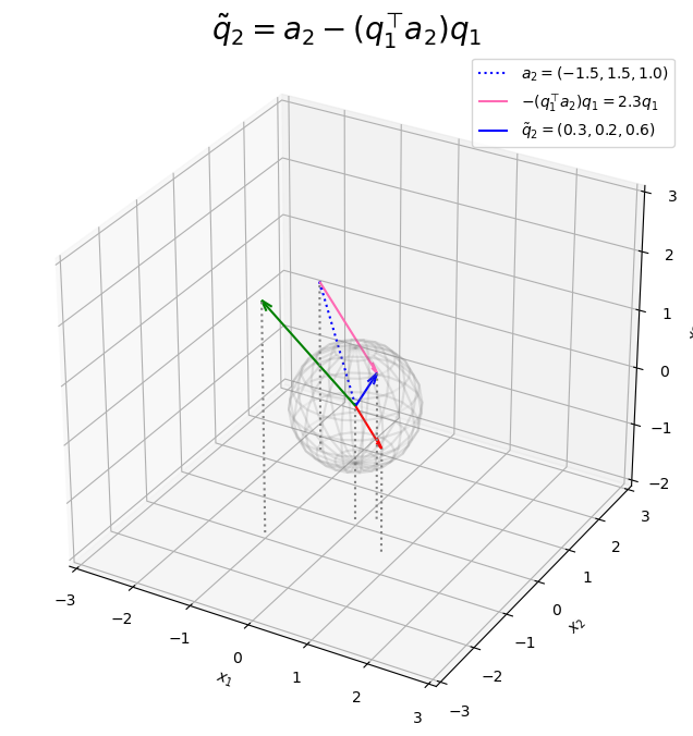
点から
移動した点が
なのが分かります。
を正規化して
とします。
# 2番目の直交ベクトルを正規化
norm_q2_tilde = np.linalg.norm(q2_tilde)
q2 = q2_tilde / norm_q2_tilde
print(q2)
print(np.linalg.norm(q2))
[0.41870402 0.26916687 0.86731548]
1.0
1番目の正規直交ベクトルのときと同様に、
で正規化します。
を描画します。
作図コード(クリックで展開)
# 2番目の正規直交ベクトルを作図
fig, ax = plt.subplots(figsize=(8, 8), facecolor='white',
                       subplot_kw={'projection': '3d'})
ax.plot_wireframe(x_grid, y_grid, z_grid,
                  color='gray', alpha=0.1) # 単位球面
ax.quiver(0, 0, 0, *a3,
          color='green', arrow_length_ratio=l/np.linalg.norm(a3)) # ベクトルa3
ax.quiver(0, 0, 0, *q1,
          color='red', arrow_length_ratio=l/np.linalg.norm(q1)) # ベクトルq1
ax.quiver(0, 0, 0, *q2_tilde,
          color='blue', linestyle=':', arrow_length_ratio=l/np.linalg.norm(q2_tilde),
          label='$\\tilde{q}_2 = ('+', '.join(map(str, q2_tilde.round(1)))+')$') # ベクトルq~2
ax.quiver(0, 0, 0, *q2,
          color='blue', arrow_length_ratio=l/np.linalg.norm(q2),
          label='$q_2 = ('+', '.join(map(str, q2.round(1)))+')$') # ベクトルq2
ax.quiver([0, a3[0], q1[0], q2_tilde[0], q2[0]],
          [0, a3[1], q1[1], q2_tilde[1], q2[1]],
          [0, a3[2], q1[2], q2_tilde[2], q2[2]],
          [0, 0, 0, 0, 0],
          [0, 0, 0, 0, 0],
          [z_min, z_min-a3[2], z_min-q1[2], z_min-q2_tilde[2], z_min-q2[2]],
          color='gray', arrow_length_ratio=0, linestyle=':') # 補助線
ax.set_xticks(ticks=np.arange(x_min, x_max+1))
ax.set_yticks(ticks=np.arange(y_min, y_max+1))
ax.set_zticks(ticks=np.arange(z_min, z_max+1))
ax.set_zlim(z_min, z_max)
ax.set_xlabel('$x_1$')
ax.set_ylabel('$x_2$')
ax.set_zlabel('$x_3$')
ax.set_title('$q_2 = \\frac{\\tilde{q}_2}{\|\\tilde{q}_2\|}$', fontsize=20)
ax.legend()
ax.set_aspect('equal')
plt.show()

が、
と同じ方向で、ノルムが1のベクトルなのが分かります。
ここまでは、2次元の場合と同じ計算でした。
続いて、の内積と
の内積を係数として、
の線形結合を
とします。
# 3番目の直交ベクトルを計算
beta1 = - np.dot(q1, a3)
beta2 = - np.dot(q2, a3)
q3_tilde = a3 + beta1 * q1 + beta2 * q2
print(q3_tilde)
[-0.97674419 -1.62790698 0.97674419]
を計算して
q3_tildeとします。
を描画します。
作図コード(クリックで展開)
# 3番目の直交ベクトルを作図
fig, ax = plt.subplots(figsize=(8, 8), facecolor='white',
                       subplot_kw={'projection': '3d'})
ax.plot_wireframe(x_grid, y_grid, z_grid,
                  color='gray', alpha=0.1) # 単位球面
ax.quiver(0, 0, 0, *a3,
          color='green', linestyle=':', arrow_length_ratio=l/np.linalg.norm(a3),
          label='$a_3=('+', '.join(map(str, a3))+')$') # ベクトルa3
ax.quiver(0, 0, 0, *q1,
          color='red', arrow_length_ratio=l/np.linalg.norm(q1)) # ベクトルq1
ax.quiver(0, 0, 0, *q2,
          color='blue', arrow_length_ratio=l/np.linalg.norm(q2)) # ベクトルq2
ax.quiver(*a3, *beta1*q1+beta2*q2,
          color='purple', arrow_length_ratio=l/np.linalg.norm(beta1*q1+beta2*q2),
          label='$- (q_1^{\\top} a_3) q_1 - (q_2^{\\top} a_3) q_2='+str(beta1.round(1))+'q_1+'+str(beta2.round(1))+'q_2$') # ベクトル-β1q1-β2q2
ax.quiver(0, 0, 0, *q3_tilde,
          color='green', arrow_length_ratio=l/np.linalg.norm(q3_tilde),
          label='$\\tilde{q}_3 = ('+', '.join(map(str, q3_tilde.round(1)))+')$') # ベクトルq~3
ax.quiver([0, a3[0], q1[0], q2[0], q3_tilde[0]],
          [0, a3[1], q1[1], q2[1], q3_tilde[1]],
          [0, a3[2], q1[2], q2[2], q3_tilde[2]],
          [0, 0, 0, 0, 0],
          [0, 0, 0, 0, 0],
          [z_min, z_min-a3[2], z_min-q1[2], z_min-q2[2], z_min-q3_tilde[2]],
          color='gray', arrow_length_ratio=0, linestyle=':') # 補助線
ax.set_xticks(ticks=np.arange(x_min, x_max+1))
ax.set_yticks(ticks=np.arange(y_min, y_max+1))
ax.set_zticks(ticks=np.arange(z_min, z_max+1))
ax.set_zlim(z_min, z_max)
ax.set_xlabel('$x_1$')
ax.set_ylabel('$x_2$')
ax.set_zlabel('$x_3$')
ax.set_title('$\\tilde{q}_3 = a_3 - (q_1^{\\top} a_3) q_1 - (q_2^{\\top} a_3) q_2$', fontsize=20)
ax.legend()
ax.set_aspect('equal')
plt.show()

点から
移動した点が
なのが分かります。
を正規化して
とします。
# 3番目の直交ベクトルを正規化
norm_q3_tilde = np.linalg.norm(q3_tilde)
q3 = q3_tilde / norm_q3_tilde
print(q3)
print(np.linalg.norm(q3))
[-0.45749571 -0.76249285  0.45749571]
1.0
ノルムで割って正規化します。
を描画します。
作図コード(クリックで展開)
# 2番目の正規直交ベクトルを作図
fig, ax = plt.subplots(figsize=(8, 8), facecolor='white',
                       subplot_kw={'projection': '3d'})
ax.plot_wireframe(x_grid, y_grid, z_grid,
                  color='gray', alpha=0.1) # 単位球面
ax.quiver(0, 0, 0, *q1,
          color='red', arrow_length_ratio=l/np.linalg.norm(q1)) # ベクトルq1
ax.quiver(0, 0, 0, *q2,
          color='blue', arrow_length_ratio=l/np.linalg.norm(q2)) # ベクトルq2
ax.quiver(0, 0, 0, *q3_tilde,
          color='green', linestyle=':', arrow_length_ratio=l/np.linalg.norm(q3_tilde),
          label='$\\tilde{q}_3 = ('+', '.join(map(str, q3_tilde.round(1)))+')$') # ベクトルq~3
ax.quiver(0, 0, 0, *q3,
          color='green', arrow_length_ratio=l/np.linalg.norm(q3),
          label='$q_3 = ('+', '.join(map(str, q3.round(1)))+')$') # ベクトルq3
ax.quiver([0, q1[0], q2[0], q3_tilde[0], q3[0]],
          [0, q1[1], q2[1], q3_tilde[1], q3[1]],
          [0, q1[2], q2[2], q3_tilde[2], q3[2]],
          [0, 0, 0, 0, 0],
          [0, 0, 0, 0, 0],
          [z_min, z_min-q1[2], z_min-q2[2], z_min-q3_tilde[2], z_min-q3[2]],
          color='gray', arrow_length_ratio=0, linestyle=':') # 補助線
ax.set_xticks(ticks=np.arange(x_min, x_max+1))
ax.set_yticks(ticks=np.arange(y_min, y_max+1))
ax.set_zticks(ticks=np.arange(z_min, z_max+1))
ax.set_zlim(z_min, z_max)
ax.set_xlabel('$x_1$')
ax.set_ylabel('$x_2$')
ax.set_zlabel('$x_3$')
ax.set_title('$q_3 = \\frac{\\tilde{q}_3}{\|\\tilde{q}_3\|}$', fontsize=20)
ax.legend()
ax.set_aspect('equal')
plt.show()

ノルムが1に正規化されているのが分かります。
最後に、が直交しているのを確認します。
# 直交しているか確認
print(np.dot(q1, q2))
print(np.dot(q2, q3))
print(np.dot(q3, q1))
3.3306690738754696e-16
0.0
-1.1102230246251565e-16
がそれぞれ正規化されているのは都度確認しました。
(プログラム上の誤差を含むことがありますが)内積が0になることから、直交しているのが分かります。
を描画します。
作図コード(クリックで展開)
# 3つの正規直交ベクトルを作図
fig, ax = plt.subplots(figsize=(8, 8), facecolor='white',
                       subplot_kw={'projection': '3d'})
ax.plot_wireframe(x_grid, y_grid, z_grid,
                  color='gray', alpha=0.1) # 単位球面
ax.quiver(0, 0, 0, *q1,
          color='red', arrow_length_ratio=l/np.linalg.norm(q1),
          label='$q_1 = ('+', '.join(map(str, q1.round(1)))+')$') # ベクトルq1
ax.quiver(0, 0, 0, *q2,
          color='blue', arrow_length_ratio=l/np.linalg.norm(q2),
          label='$q_2 = ('+', '.join(map(str, q2.round(1)))+')$') # ベクトルq2
ax.quiver(0, 0, 0, *q3,
          color='green', arrow_length_ratio=l/np.linalg.norm(q3),
          label='$q_3 = ('+', '.join(map(str, q3.round(1)))+')$') # ベクトルq3
ax.quiver([0, q1[0], q2[0], q3[0]],
          [0, q1[1], q2[1], q3[1]],
          [0, q1[2], q2[2], q3[2]],
          [0, 0, 0, 0],
          [0, 0, 0, 0],
          [z_min, z_min-q1[2], z_min-q2[2], z_min-q3[2]],
          color='gray', arrow_length_ratio=0, linestyle=':') # 補助線
ax.set_xticks(ticks=np.arange(x_min, x_max+1))
ax.set_yticks(ticks=np.arange(y_min, y_max+1))
ax.set_zticks(ticks=np.arange(z_min, z_max+1))
ax.set_zlim(z_min, z_max)
ax.set_xlabel('$x_1$')
ax.set_ylabel('$x_2$')
ax.set_zlabel('$x_3$')
ax.set_title('$q_1 \\bot q_2, q_2 \\bot q_3, q_3 \\bot q_1$', fontsize=20)
ax.legend()
ax.set_aspect('equal')
plt.show()

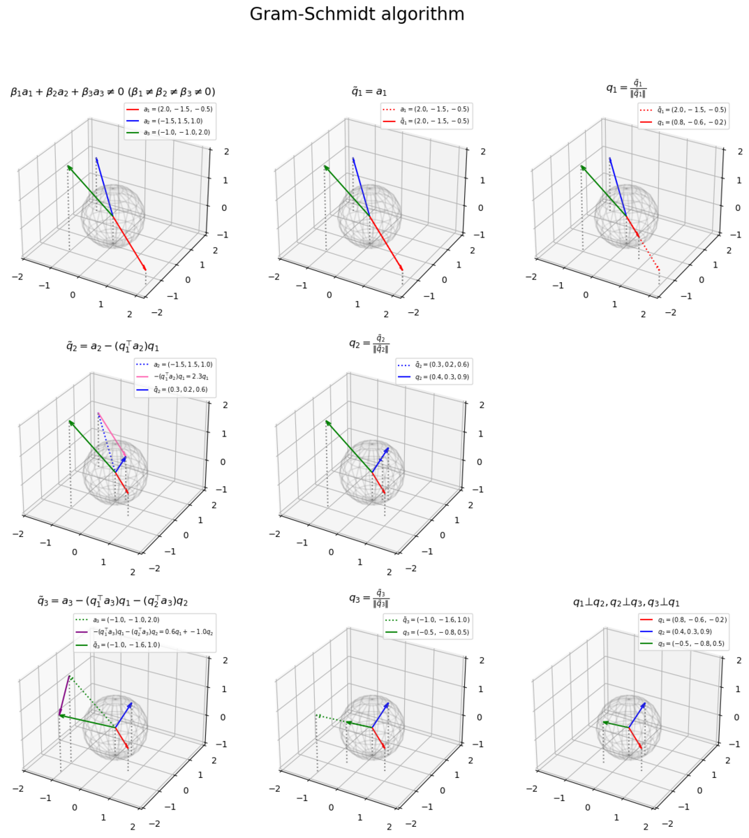
以上で、グラム・シュミット法により、3次元空間における3つの正規直交ベクトルが得られました。
正規直交化の可視化
正規直交化の処理をまとめて行います。
作図コード(クリックで展開)
3つの正規直交ベクトルをまとめて計算します。
# ベクトルを指定
a1 = np.array([2.0, -1.5, -0.5])
a2 = np.array([-1.5, 1.5, 1.0])
a3 = np.array([-1.0, -1.0, 2.0])


# 1番目のベクトルを複製(1番目の直交ベクトルを作成)
q1_tilde = a1.copy()

# 1番目の直交ベクトルを正規化
norm_q1_tilde = np.linalg.norm(q1_tilde)
q1 = q1_tilde / norm_q1_tilde

# 2番目の直交ベクトルを計算
beta21 = - np.dot(q1, a2)
q2_tilde = a2 + beta21 * q1

# 2番目の直交ベクトルを正規化
norm_q2_tilde = np.linalg.norm(q2_tilde)
q2 = q2_tilde / norm_q2_tilde

# 3番目の直交ベクトルを計算
beta31 = - np.dot(q1, a3)
beta32 = - np.dot(q2, a3)
q3_tilde = a3 + beta31 * q1 + beta32 * q2

# 3番目の直交ベクトルを正規化
norm_q3_tilde = np.linalg.norm(q3_tilde)
q3 = q3_tilde / norm_q3_tilde
係数の変数名が干渉しないように、の計算における変数名を
beta21、の計算における変数名を
beta31, beta32に変更しました。
8枚のグラフ(計算)をまとめて作図します。
# グラフサイズ用の値を設定
x_min = np.floor(np.min([0.0, a1[0], a2[0], a3[0]]))
x_max = np.ceil(np.max([0.0, a1[0], a2[0], a3[0]]))
y_min = np.floor(np.min([0.0, a1[1], a2[1], a3[1]]))
y_max = np.ceil(np.max([0.0, a1[1], a2[1], a3[1]]))
z_min = np.floor(np.min([0.0, a1[2], a2[2], a3[2]]))
z_max = np.ceil(np.max([0.0, a1[2], a2[2], a3[2]]))

# 矢印のサイズを指定
l = 0.2

# 凡例の表示位置を指定
loc_str = 'upper right'

# グラム・シュミッド法の作図
fig, axes = plt.subplots(nrows=3, ncols=3, figsize=(15, 15), facecolor='white',
                         subplot_kw={'projection': '3d'})
fig.suptitle('Gram-Schmidt algorithm', fontsize=20)

# 元のベクトルを作図
axes[0, 0].plot_wireframe(x_grid, y_grid, z_grid,
                          color='gray', alpha=0.1) # 単位球
axes[0, 0].quiver(0, 0, 0, *a1,
                  color='red', arrow_length_ratio=l/np.linalg.norm(a1),
                  label='$a_1 = ('+', '.join(map(str, a1))+')$') # ベクトルa1
axes[0, 0].quiver(0, 0, 0, *a2,
                  color='blue', arrow_length_ratio=l/np.linalg.norm(a2),
                  label='$a_2 = ('+', '.join(map(str, a2))+')$') # ベクトルa2
axes[0, 0].quiver(0, 0, 0, *a3,
                  color='green', arrow_length_ratio=l/np.linalg.norm(a3),
                  label='$a_3 = ('+', '.join(map(str, a3))+')$') # ベクトルa3
axes[0, 0].quiver([0, a1[0], a2[0], a3[0]],
                  [0, a1[1], a2[1], a3[1]],
                  [0, a1[2], a2[2], a3[2]],
                  [0, 0, 0, 0],
                  [0, 0, 0, 0],
                  [z_min, z_min-a1[2], z_min-a2[2], z_min-a3[2]],
                  color='gray', arrow_length_ratio=0, linestyle=':') # 補助線
axes[0, 0].set_xticks(ticks=np.arange(x_min, x_max+1))
axes[0, 0].set_yticks(ticks=np.arange(y_min, y_max+1))
axes[0, 0].set_zticks(ticks=np.arange(z_min, z_max+1))
axes[0, 0].set_zlim(z_min, z_max)
axes[0, 0].set_title('$\\beta_1 a_1 + \\beta_2 a_2 + \\beta_3 a_3 \\neq 0\ (\\beta_1 \\neq \\beta_2 \\neq \\beta_3 \\neq 0)$')
axes[0, 0].legend(loc=loc_str, prop={'size': 7})
axes[0, 0].set_aspect('equal')

# 1番目の直交ベクトルを作図
axes[0, 1].plot_wireframe(x_grid, y_grid, z_grid,
                          color='gray', alpha=0.1) # 単位球
axes[0, 1].quiver(0, 0, 0, *a1,
                  color='red', linestyle=':', arrow_length_ratio=l/np.linalg.norm(a1),
                  label='$a_1 = ('+', '.join(map(str, a1))+')$') # ベクトルa1
axes[0, 1].quiver(0, 0, 0, *a2,
                  color='blue', arrow_length_ratio=l/np.linalg.norm(a2)) # ベクトルa2
axes[0, 1].quiver(0, 0, 0, *a3,
                  color='green', arrow_length_ratio=l/np.linalg.norm(a3)) # ベクトルa3
axes[0, 1].quiver(0, 0, 0, *q1_tilde,
                  color='red', arrow_length_ratio=l/np.linalg.norm(q1_tilde),
                  label='$\\tilde{q}_1 = ('+', '.join(map(str, q1_tilde))+')$') # ベクトルq~1
axes[0, 1].quiver([0, a1[0], a2[0], a3[0], q1_tilde[0]],
                  [0, a1[1], a2[1], a3[1], q1_tilde[1]],
                  [0, a1[2], a2[2], a3[2], q1_tilde[2]],
                  [0, 0, 0, 0, 0],
                  [0, 0, 0, 0, 0],
                  [z_min, z_min-a1[2], z_min-a2[2], z_min-a3[2], z_min-q1_tilde[2]],
                  color='gray', arrow_length_ratio=0, linestyle=':') # 補助線
axes[0, 1].set_xticks(ticks=np.arange(x_min, x_max+1))
axes[0, 1].set_yticks(ticks=np.arange(y_min, y_max+1))
axes[0, 1].set_zticks(ticks=np.arange(z_min, z_max+1))
axes[0, 1].set_zlim(z_min, z_max)
axes[0, 1].set_title('$\\tilde{q}_1 = a_1$')
axes[0, 1].legend(loc=loc_str, prop={'size': 7})
axes[0, 1].set_aspect('equal')

# 1番目の正規直交ベクトルを作図
axes[0, 2].plot_wireframe(x_grid, y_grid, z_grid,
                          color='gray', alpha=0.1) # 単位球
axes[0, 2].quiver(0, 0, 0, *a2,
                  color='blue', arrow_length_ratio=l/np.linalg.norm(a2)) # ベクトルa2
axes[0, 2].quiver(0, 0, 0, *a3,
                  color='green', arrow_length_ratio=l/np.linalg.norm(a3)) # ベクトルa3
axes[0, 2].quiver(0, 0, 0, *q1_tilde,
                  color='red', linestyle=':', arrow_length_ratio=l/np.linalg.norm(q1_tilde),
                  label='$\\tilde{q}_1 = ('+', '.join(map(str, q1_tilde))+')$') # ベクトルq~1
axes[0, 2].quiver(0, 0, 0, *q1,
                  color='red', arrow_length_ratio=l/np.linalg.norm(q1),
                  label='$q_1 = ('+', '.join(map(str, q1.round(1)))+')$') # ベクトルq1
axes[0, 2].quiver([0, a2[0], a3[0], q1_tilde[0], q1[0]],
                  [0, a2[1], a3[1], q1_tilde[1], q1[1]],
                  [0, a2[2], a3[2], q1_tilde[2], q1[2]],
                  [0, 0, 0, 0, 0],
                  [0, 0, 0, 0, 0],
                  [z_min, z_min-a2[2], z_min-a3[2], z_min-q1_tilde[2], z_min-q1[2]],
                  color='gray', arrow_length_ratio=0, linestyle=':') # 補助線
axes[0, 2].set_xticks(ticks=np.arange(x_min, x_max+1))
axes[0, 2].set_yticks(ticks=np.arange(y_min, y_max+1))
axes[0, 2].set_zticks(ticks=np.arange(z_min, z_max+1))
axes[0, 2].set_zlim(z_min, z_max)
axes[0, 2].set_title('$q_1 = \\frac{\\tilde{q}_1}{\|\\tilde{q}_1\|}$')
axes[0, 2].legend(loc=loc_str, prop={'size': 7})
axes[0, 2].set_aspect('equal')

# 2番目の直交ベクトルを作図
axes[1, 0].plot_wireframe(x_grid, y_grid, z_grid,
                          color='gray', alpha=0.1) # 単位球
axes[1, 0].quiver(0, 0, 0, *a2,
                  color='blue', linestyle=':', arrow_length_ratio=l/np.linalg.norm(a2),
                  label='$a_2=('+', '.join(map(str, a2))+')$') # ベクトルa2
axes[1, 0].quiver(0, 0, 0, *a3,
                  color='green', arrow_length_ratio=l/np.linalg.norm(a3)) # ベクトルa3
axes[1, 0].quiver(0, 0, 0, *q1,
                  color='red', arrow_length_ratio=l/np.linalg.norm(q1)) # ベクトルq1
axes[1, 0].quiver(*a2, *beta21*q1,
                  color='hotpink', arrow_length_ratio=l/np.linalg.norm(beta21*q1),
                  label='$- (q_1^{\\top} a_2) q_1='+str(beta21.round(1))+'q_1$') # ベクトル-β1q1
axes[1, 0].quiver(0, 0, 0, *q2_tilde,
                  color='blue', arrow_length_ratio=l/np.linalg.norm(q2_tilde),
                  label='$\\tilde{q}_2 = ('+', '.join(map(str, q2_tilde.round(1)))+')$') # ベクトルq~2
axes[1, 0].quiver([0, a2[0], a3[0], q1[0], q2_tilde[0]],
                  [0, a2[1], a3[1], q1[1], q2_tilde[1]],
                  [0, a2[2], a3[2], q1[2], q2_tilde[2]],
                  [0, 0, 0, 0, 0],
                  [0, 0, 0, 0, 0],
                  [z_min, z_min-a2[2], z_min-a3[2], z_min-q1[2], z_min-q2_tilde[2]],
                  color='gray', arrow_length_ratio=0, linestyle=':') # 補助線
axes[1, 0].set_xticks(ticks=np.arange(x_min, x_max+1))
axes[1, 0].set_yticks(ticks=np.arange(y_min, y_max+1))
axes[1, 0].set_zticks(ticks=np.arange(z_min, z_max+1))
axes[1, 0].set_zlim(z_min, z_max)
axes[1, 0].set_title('$\\tilde{q}_2 = a_2 - (q_1^{\\top} a_2) q_1$')
axes[1, 0].legend(loc=loc_str, prop={'size': 7})
axes[1, 0].set_aspect('equal')

# 2番目の正規直交ベクトルを作図
axes[1, 1].plot_wireframe(x_grid, y_grid, z_grid,
                          color='gray', alpha=0.1) # 単位球
axes[1, 1].quiver(0, 0, 0, *a3,
                  color='green', arrow_length_ratio=l/np.linalg.norm(a3)) # ベクトルa3
axes[1, 1].quiver(0, 0, 0, *q1,
                  color='red', arrow_length_ratio=l/np.linalg.norm(q1)) # ベクトルq1
axes[1, 1].quiver(0, 0, 0, *q2_tilde,
                  color='blue', linestyle=':', arrow_length_ratio=l/np.linalg.norm(q2_tilde),
                  label='$\\tilde{q}_2 = ('+', '.join(map(str, q2_tilde.round(1)))+')$') # ベクトルq~2
axes[1, 1].quiver(0, 0, 0, *q2,
                  color='blue', arrow_length_ratio=l/np.linalg.norm(q2),
                  label='$q_2 = ('+', '.join(map(str, q2.round(1)))+')$') # ベクトルq2
axes[1, 1].quiver([0, a3[0], q1[0], q2_tilde[0], q2[0]],
                  [0, a3[1], q1[1], q2_tilde[1], q2[1]],
                  [0, a3[2], q1[2], q2_tilde[2], q2[2]],
                  [0, 0, 0, 0, 0],
                  [0, 0, 0, 0, 0],
                  [z_min, z_min-a3[2], z_min-q1[2], z_min-q2_tilde[2], z_min-q2[2]],
                  color='gray', arrow_length_ratio=0, linestyle=':') # 補助線
axes[1, 1].set_xticks(ticks=np.arange(x_min, x_max+1))
axes[1, 1].set_yticks(ticks=np.arange(y_min, y_max+1))
axes[1, 1].set_zticks(ticks=np.arange(z_min, z_max+1))
axes[1, 1].set_zlim(z_min, z_max)
axes[1, 1].set_title('$q_2 = \\frac{\\tilde{q}_2}{\|\\tilde{q}_2\|}$')
axes[1, 1].legend(loc=loc_str, prop={'size': 7})
axes[1, 1].set_aspect('equal')

# 不要なグラフを非表示
axes[1, 2].axis('off')

# 3番目の直交ベクトルを作図
axes[2, 0].plot_wireframe(x_grid, y_grid, z_grid,
                          color='gray', alpha=0.1) # 単位球
axes[2, 0].quiver(0, 0, 0, *a3,
                  color='green', linestyle=':', arrow_length_ratio=l/np.linalg.norm(a3),
                  label='$a_3=('+', '.join(map(str, a3))+')$') # ベクトルa3
axes[2, 0].quiver(0, 0, 0, *q1,
                  color='red', arrow_length_ratio=l/np.linalg.norm(q1)) # ベクトルq1
axes[2, 0].quiver(0, 0, 0, *q2,
                  color='blue', arrow_length_ratio=l/np.linalg.norm(q2)) # ベクトルq2
axes[2, 0].quiver(*a3, *beta31*q1+beta32*q2,
                  color='purple', arrow_length_ratio=l/np.linalg.norm(beta31*q1+beta32*q2),
                  label='$- (q_1^{\\top} a_3) q_1 - (q_2^{\\top} a_3) q_2='+str(beta31.round(1))+'q_1+'+str(beta32.round(1))+'q_2$') # ベクトル-β1q1-β2q2
axes[2, 0].quiver(0, 0, 0, *q3_tilde,
                  color='green', arrow_length_ratio=l/np.linalg.norm(q3_tilde),
                  label='$\\tilde{q}_3 = ('+', '.join(map(str, q3_tilde.round(1)))+')$') # ベクトルq~3
axes[2, 0].quiver([0, a3[0], q1[0], q2[0], q3_tilde[0]],
                  [0, a3[1], q1[1], q2[1], q3_tilde[1]],
                  [0, a3[2], q1[2], q2[2], q3_tilde[2]],
                  [0, 0, 0, 0, 0],
                  [0, 0, 0, 0, 0],
                  [z_min, z_min-a3[2], z_min-q1[2], z_min-q2[2], z_min-q3_tilde[2]],
                  color='gray', arrow_length_ratio=0, linestyle=':') # 補助線
axes[2, 0].set_xticks(ticks=np.arange(x_min, x_max+1))
axes[2, 0].set_yticks(ticks=np.arange(y_min, y_max+1))
axes[2, 0].set_zticks(ticks=np.arange(z_min, z_max+1))
axes[2, 0].set_zlim(z_min, z_max)
axes[2, 0].set_title('$\\tilde{q}_3 = a_3 - (q_1^{\\top} a_3) q_1 - (q_2^{\\top} a_3) q_2$')
axes[2, 0].legend(loc=loc_str, prop={'size': 7})
axes[2, 0].set_aspect('equal')

# 2番目の正規直交ベクトルを作図
axes[2, 1].plot_wireframe(x_grid, y_grid, z_grid,
                          color='gray', alpha=0.1) # 単位球
axes[2, 1].quiver(0, 0, 0, *q1,
                  color='red', arrow_length_ratio=l/np.linalg.norm(q1)) # ベクトルq1
axes[2, 1].quiver(0, 0, 0, *q2,
                  color='blue', arrow_length_ratio=l/np.linalg.norm(q2)) # ベクトルq2
axes[2, 1].quiver(0, 0, 0, *q3_tilde,
                  color='green', linestyle=':', arrow_length_ratio=l/np.linalg.norm(q3_tilde),
                  label='$\\tilde{q}_3 = ('+', '.join(map(str, q3_tilde.round(1)))+')$') # ベクトルq~3
axes[2, 1].quiver(0, 0, 0, *q3,
                  color='green', arrow_length_ratio=l/np.linalg.norm(q3),
                  label='$q_3 = ('+', '.join(map(str, q3.round(1)))+')$') # ベクトルq3
axes[2, 1].quiver([0, q1[0], q2[0], q3_tilde[0], q3[0]],
                  [0, q1[1], q2[1], q3_tilde[1], q3[1]],
                  [0, q1[2], q2[2], q3_tilde[2], q3[2]],
                  [0, 0, 0, 0, 0],
                  [0, 0, 0, 0, 0],
                  [z_min, z_min-q1[2], z_min-q2[2], z_min-q3_tilde[2], z_min-q3[2]],
                  color='gray', arrow_length_ratio=0, linestyle=':') # 補助線
axes[2, 1].set_xticks(ticks=np.arange(x_min, x_max+1))
axes[2, 1].set_yticks(ticks=np.arange(y_min, y_max+1))
axes[2, 1].set_zticks(ticks=np.arange(z_min, z_max+1))
axes[2, 1].set_zlim(z_min, z_max)
axes[2, 1].set_title('$q_3 = \\frac{\\tilde{q}_3}{\|\\tilde{q}_3\|}$')
axes[2, 1].legend(loc=loc_str, prop={'size': 7})
axes[2, 1].set_aspect('equal')

# 3つの正規直交ベクトルを作図
axes[2, 2].plot_wireframe(x_grid, y_grid, z_grid,
                          color='gray', alpha=0.1) # 単位球
axes[2, 2].quiver(0, 0, 0, *q1,
                  color='red', arrow_length_ratio=l/np.linalg.norm(q1),
                  label='$q_1 = ('+', '.join(map(str, q1.round(1)))+')$') # ベクトルq1
axes[2, 2].quiver(0, 0, 0, *q2,
                  color='blue', arrow_length_ratio=l/np.linalg.norm(q2),
                  label='$q_2 = ('+', '.join(map(str, q2.round(1)))+')$') # ベクトルq2
axes[2, 2].quiver(0, 0, 0, *q3,
                  color='green', arrow_length_ratio=l/np.linalg.norm(q3),
                  label='$q_3 = ('+', '.join(map(str, q3.round(1)))+')$') # ベクトルq3
axes[2, 2].quiver([0, q1[0], q2[0], q3[0]],
                  [0, q1[1], q2[1], q3[1]],
                  [0, q1[2], q2[2], q3[2]],
                  [0, 0, 0, 0],
                  [0, 0, 0, 0],
                  [z_min, z_min-q1[2], z_min-q2[2], z_min-q3[2]],
                  color='gray', arrow_length_ratio=0, linestyle=':') # 補助線
axes[2, 2].set_xticks(ticks=np.arange(x_min, x_max+1))
axes[2, 2].set_yticks(ticks=np.arange(y_min, y_max+1))
axes[2, 2].set_zticks(ticks=np.arange(z_min, z_max+1))
axes[2, 2].set_zlim(z_min, z_max)
axes[2, 2].set_title('$q_1 \\bot q_2, q_2 \\bot q_3, q_3 \\bot q_1$')
axes[2, 2].legend(loc=loc_str, prop={'size': 7})
axes[2, 2].set_aspect('equal')

plt.show()
plt.subplots()の行数の引数nrowsと列数の引数ncolsを指定して、9個分のグラフオブジェクトをaxesとして、それぞれ「正規直交ベクトルの計算」の作図処理を行います。
不要なグラフの場合は、axes.axis('off')で軸を非表示にします。
ベクトルの値を変化させたアニメーションを作成します。
作図コード(クリックで展開)
# フレーム数を設定
frame_num = 51

# 各次元の要素として利用する値を指定
a1_vals = np.array(
    [np.linspace(start=-1.0, stop=2.0, num=frame_num),
     np.linspace(start=-1.5, stop=2.0, num=frame_num),
     np.linspace(start=-2.0, stop=2.0, num=frame_num)]
).T
a2_vals = np.array(
    [np.linspace(start=0.6, stop=-1.2, num=frame_num),
     np.linspace(start=-0.5, stop=1.5, num=frame_num),
     np.linspace(start=1.6, stop=1.6, num=frame_num)]
).T
a3_vals = np.array(
    [np.linspace(start=-1.0, stop=-1.0, num=frame_num),
     np.linspace(start=-1.0, stop=-1.0, num=frame_num),
     np.linspace(start=1.9, stop=1.9, num=frame_num)]
).T

# グラフサイズ用の値を設定
x_min = np.floor(np.min([-1.0, *a1_vals[:, 0], *a2_vals[:, 0], *a3_vals[:, 0]]))
x_max = np.ceil(np.max([1.0, *a1_vals[:, 0], *a2_vals[:, 0], *a3_vals[:, 0]]))
y_min = np.floor(np.min([-1.0, *a1_vals[:, 1], *a2_vals[:, 1], *a3_vals[:, 1]]))
y_max = np.ceil(np.max([1.0, *a1_vals[:, 1], *a2_vals[:, 1], *a3_vals[:, 1]]))
z_min = np.floor(np.min([-1.0, *a1_vals[:, 2], *a2_vals[:, 2], *a3_vals[:, 2]]))
z_max = np.ceil(np.max([1.0, *a1_vals[:, 2], *a2_vals[:, 2], *a3_vals[:, 2]]))

# 矢印のサイズを指定
l = 0.2

# 凡例の表示位置を指定
loc_str = 'upper left'

# グラム・シュミッド法の作図
fig, axes = plt.subplots(nrows=3, ncols=3, figsize=(18, 18), facecolor='white',
                         subplot_kw={'projection': '3d'})
fig.suptitle('Gram-Schmidt algorithm', fontsize=20)

# 作図処理を関数として定義
def update(i):

    # i番目のベクトルを作成
    a1 = a1_vals[i]
    a2 = a2_vals[i]
    a3 = a3_vals[i]

    # 1番目のベクトルを複製(1番目の直交ベクトルを作成)
    q1_tilde = a1.copy()

    # 1番目の直交ベクトルを正規化
    norm_q1_tilde = np.linalg.norm(q1_tilde)
    q1 = q1_tilde / norm_q1_tilde

    # 2番目の直交ベクトルを計算
    beta21 = - np.dot(q1, a2)
    q2_tilde = a2 + beta21 * q1

    # 2番目の直交ベクトルを正規化
    norm_q2_tilde = np.linalg.norm(q2_tilde)
    q2 = q2_tilde / norm_q2_tilde

    # 3番目の直交ベクトルを計算
    beta31 = - np.dot(q1, a3)
    beta32 = - np.dot(q2, a3)
    q3_tilde = a3 + beta31 * q1 + beta32 * q2

    # 3番目の直交ベクトルを正規化
    norm_q3_tilde = np.linalg.norm(q3_tilde)
    q3 = q3_tilde / norm_q3_tilde

    # 元のベクトルを作図
    axes[0, 0].clear() # 前フレームのグラフを初期化
    axes[0, 0].plot_wireframe(x_grid, y_grid, z_grid,
                              color='gray', alpha=0.1) # 単位球
    axes[0, 0].quiver(0, 0, 0, *a1,
                      color='red', arrow_length_ratio=l/np.linalg.norm(a1),
                      label='$a_1 = ('+', '.join(map(str, a1.round(1)))+')$') # ベクトルa1
    axes[0, 0].quiver(0, 0, 0, *a2,
                      color='blue', arrow_length_ratio=l/np.linalg.norm(a2),
                      label='$a_2 = ('+', '.join(map(str, a2.round(1)))+')$') # ベクトルa2
    axes[0, 0].quiver(0, 0, 0, *a3,
                      color='green', arrow_length_ratio=l/np.linalg.norm(a3),
                      label='$a_3 = ('+', '.join(map(str, a3.round(1)))+')$') # ベクトルa3
    axes[0, 0].quiver([0, a1[0], a2[0], a3[0]],
                      [0, a1[1], a2[1], a3[1]],
                      [0, a1[2], a2[2], a3[2]],
                      [0, 0, 0, 0],
                      [0, 0, 0, 0],
                      [z_min, z_min-a1[2], z_min-a2[2], z_min-a3[2]],
                      color='gray', arrow_length_ratio=0, linestyle=':') # 補助線
    axes[0, 0].set_xticks(ticks=np.arange(x_min, x_max+1))
    axes[0, 0].set_yticks(ticks=np.arange(y_min, y_max+1))
    axes[0, 0].set_zticks(ticks=np.arange(z_min, z_max+1))
    axes[0, 0].set_xlim(x_min, x_max)
    axes[0, 0].set_ylim(y_min, y_max)
    axes[0, 0].set_zlim(z_min, z_max)
    axes[0, 0].set_title('$\\beta_1 a_1 + \\beta_2 a_2 + \\beta_3 a_3 \\neq 0\ (\\beta_1 \\neq \\beta_2 \\neq \\beta_3 \\neq 0)$')
    axes[0, 0].legend(loc=loc_str, prop={'size': 7})
    axes[0, 0].set_aspect('equal')

    # 1番目の直交ベクトルを作図
    axes[0, 1].clear() # 前フレームのグラフを初期化
    axes[0, 1].plot_wireframe(x_grid, y_grid, z_grid,
                              color='gray', alpha=0.1) # 単位球
    axes[0, 1].quiver(0, 0, 0, *a1,
                      color='red', linestyle=':', arrow_length_ratio=l/np.linalg.norm(a1),
                      label='$a_1 = ('+', '.join(map(str, a1.round(1)))+')$') # ベクトルa1
    axes[0, 1].quiver(0, 0, 0, *a2,
                      color='blue', arrow_length_ratio=l/np.linalg.norm(a2)) # ベクトルa2
    axes[0, 1].quiver(0, 0, 0, *a3,
                      color='green', arrow_length_ratio=l/np.linalg.norm(a3)) # ベクトルa3
    axes[0, 1].quiver(0, 0, 0, *q1_tilde,
                      color='red', arrow_length_ratio=l/np.linalg.norm(q1_tilde),
                      label='$\\tilde{q}_1 = ('+', '.join(map(str, q1_tilde.round(1)))+')$') # ベクトルq~1
    axes[0, 1].quiver([0, a1[0], a2[0], a3[0], q1_tilde[0]],
                      [0, a1[1], a2[1], a3[1], q1_tilde[1]],
                      [0, a1[2], a2[2], a3[2], q1_tilde[2]],
                      [0, 0, 0, 0, 0],
                      [0, 0, 0, 0, 0],
                      [z_min, z_min-a1[2], z_min-a2[2], z_min-a3[2], z_min-q1_tilde[2]],
                      color='gray', arrow_length_ratio=0, linestyle=':') # 補助線
    axes[0, 1].set_xticks(ticks=np.arange(x_min, x_max+1))
    axes[0, 1].set_yticks(ticks=np.arange(y_min, y_max+1))
    axes[0, 1].set_zticks(ticks=np.arange(z_min, z_max+1))
    axes[0, 1].set_xlim(x_min, x_max)
    axes[0, 1].set_ylim(y_min, y_max)
    axes[0, 1].set_zlim(z_min, z_max)
    axes[0, 1].set_title('$\\tilde{q}_1 = a_1$')
    axes[0, 1].legend(loc=loc_str, prop={'size': 7})
    axes[0, 1].set_aspect('equal')

    # 1番目の正規直交ベクトルを作図
    axes[0, 2].clear() # 前フレームのグラフを初期化
    axes[0, 2].plot_wireframe(x_grid, y_grid, z_grid,
                              color='gray', alpha=0.1) # 単位球
    axes[0, 2].quiver(0, 0, 0, *a2,
                      color='blue', arrow_length_ratio=l/np.linalg.norm(a2)) # ベクトルa2
    axes[0, 2].quiver(0, 0, 0, *a3,
                      color='green', arrow_length_ratio=l/np.linalg.norm(a3)) # ベクトルa3
    axes[0, 2].quiver(0, 0, 0, *q1_tilde,
                      color='red', linestyle=':', arrow_length_ratio=l/np.linalg.norm(q1_tilde),
                      label='$\\tilde{q}_1 = ('+', '.join(map(str, q1_tilde.round(1)))+')$') # ベクトルq~1
    axes[0, 2].quiver(0, 0, 0, *q1,
                      color='red', arrow_length_ratio=l/np.linalg.norm(q1),
                      label='$q_1 = ('+', '.join(map(str, q1.round(1)))+')$') # ベクトルq1
    axes[0, 2].quiver([0, a2[0], a3[0], q1_tilde[0], q1[0]],
                      [0, a2[1], a3[1], q1_tilde[1], q1[1]],
                      [0, a2[2], a3[2], q1_tilde[2], q1[2]],
                      [0, 0, 0, 0, 0],
                      [0, 0, 0, 0, 0],
                      [z_min, z_min-a2[2], z_min-a3[2], z_min-q1_tilde[2], z_min-q1[2]],
                      color='gray', arrow_length_ratio=0, linestyle=':') # 補助線
    axes[0, 2].set_xticks(ticks=np.arange(x_min, x_max+1))
    axes[0, 2].set_yticks(ticks=np.arange(y_min, y_max+1))
    axes[0, 2].set_zticks(ticks=np.arange(z_min, z_max+1))
    axes[0, 2].set_xlim(x_min, x_max)
    axes[0, 2].set_ylim(y_min, y_max)
    axes[0, 2].set_zlim(z_min, z_max)
    axes[0, 2].set_title('$q_1 = \\frac{\\tilde{q}_1}{\|\\tilde{q}_1\|}$')
    axes[0, 2].legend(loc=loc_str, prop={'size': 7})
    axes[0, 2].set_aspect('equal')

    # 2番目の直交ベクトルを作図
    axes[1, 0].clear() # 前フレームのグラフを初期化
    axes[1, 0].plot_wireframe(x_grid, y_grid, z_grid,
                              color='gray', alpha=0.1) # 単位球
    axes[1, 0].quiver(0, 0, 0, *a2,
                      color='blue', linestyle=':', arrow_length_ratio=l/np.linalg.norm(a2),
                      label='$a_2=('+', '.join(map(str, a2.round(1)))+')$') # ベクトルa2
    axes[1, 0].quiver(0, 0, 0, *a3,
                      color='green', arrow_length_ratio=l/np.linalg.norm(a3)) # ベクトルa3
    axes[1, 0].quiver(0, 0, 0, *q1,
                      color='red', arrow_length_ratio=l/np.linalg.norm(q1)) # ベクトルq1
    axes[1, 0].quiver(*a2, *beta21*q1,
                      color='hotpink', arrow_length_ratio=l/np.linalg.norm(beta21*q1),
                      label='$- (q_1^{\\top} a_2) q_1='+str(beta21.round(1))+'q_1$') # ベクトル-β1q1
    axes[1, 0].quiver(0, 0, 0, *q2_tilde,
                      color='blue', arrow_length_ratio=l/np.linalg.norm(q2_tilde),
                      label='$\\tilde{q}_2 = ('+', '.join(map(str, q2_tilde.round(1)))+')$') # ベクトルq~2
    axes[1, 0].quiver([0, a2[0], a3[0], q1[0], q2_tilde[0]],
                      [0, a2[1], a3[1], q1[1], q2_tilde[1]],
                      [0, a2[2], a3[2], q1[2], q2_tilde[2]],
                      [0, 0, 0, 0, 0],
                      [0, 0, 0, 0, 0],
                      [z_min, z_min-a2[2], z_min-a3[2], z_min-q1[2], z_min-q2_tilde[2]],
                      color='gray', arrow_length_ratio=0, linestyle=':') # 補助線
    axes[1, 0].set_xticks(ticks=np.arange(x_min, x_max+1))
    axes[1, 0].set_yticks(ticks=np.arange(y_min, y_max+1))
    axes[1, 0].set_zticks(ticks=np.arange(z_min, z_max+1))
    axes[1, 0].set_xlim(x_min, x_max)
    axes[1, 0].set_ylim(y_min, y_max)
    axes[1, 0].set_zlim(z_min, z_max)
    axes[1, 0].set_title('$\\tilde{q}_2 = a_2 - (q_1^{\\top} a_2) q_1$')
    axes[1, 0].legend(loc=loc_str, prop={'size': 7})
    axes[1, 0].set_aspect('equal')

    # 2番目の正規直交ベクトルを作図
    axes[1, 1].clear() # 前フレームのグラフを初期化
    axes[1, 1].plot_wireframe(x_grid, y_grid, z_grid,
                              color='gray', alpha=0.1) # 単位球
    axes[1, 1].quiver(0, 0, 0, *a3,
                      color='green', arrow_length_ratio=l/np.linalg.norm(a3)) # ベクトルa3
    axes[1, 1].quiver(0, 0, 0, *q1,
                      color='red', arrow_length_ratio=l/np.linalg.norm(q1)) # ベクトルq1
    axes[1, 1].quiver(0, 0, 0, *q2_tilde,
                      color='blue', linestyle=':', arrow_length_ratio=l/np.linalg.norm(q2_tilde),
                      label='$\\tilde{q}_2 = ('+', '.join(map(str, q2_tilde.round(1)))+')$') # ベクトルq~2
    axes[1, 1].quiver(0, 0, 0, *q2,
                      color='blue', arrow_length_ratio=l/np.linalg.norm(q2),
                      label='$q_2 = ('+', '.join(map(str, q2.round(1)))+')$') # ベクトルq2
    axes[1, 1].quiver([0, a3[0], q1[0], q2_tilde[0], q2[0]],
                      [0, a3[1], q1[1], q2_tilde[1], q2[1]],
                      [0, a3[2], q1[2], q2_tilde[2], q2[2]],
                      [0, 0, 0, 0, 0],
                      [0, 0, 0, 0, 0],
                      [z_min, z_min-a3[2], z_min-q1[2], z_min-q2_tilde[2], z_min-q2[2]],
                      color='gray', arrow_length_ratio=0, linestyle=':') # 補助線
    axes[1, 1].set_xticks(ticks=np.arange(x_min, x_max+1))
    axes[1, 1].set_yticks(ticks=np.arange(y_min, y_max+1))
    axes[1, 1].set_zticks(ticks=np.arange(z_min, z_max+1))
    axes[1, 1].set_xlim(x_min, x_max)
    axes[1, 1].set_ylim(y_min, y_max)
    axes[1, 1].set_zlim(z_min, z_max)
    axes[1, 1].set_title('$q_2 = \\frac{\\tilde{q}_2}{\|\\tilde{q}_2\|}$')
    axes[1, 1].legend(loc=loc_str, prop={'size': 7})
    axes[1, 1].set_aspect('equal')

    # 不要なグラフを非表示
    axes[1, 2].axis('off')

    # 3番目の直交ベクトルを作図
    axes[2, 0].clear() # 前フレームのグラフを初期化
    axes[2, 0].plot_wireframe(x_grid, y_grid, z_grid,
                              color='gray', alpha=0.1) # 単位球
    axes[2, 0].quiver(0, 0, 0, *a3,
                      color='green', linestyle=':', arrow_length_ratio=l/np.linalg.norm(a3),
                      label='$a_3=('+', '.join(map(str, a3.round(1)))+')$') # ベクトルa3
    axes[2, 0].quiver(0, 0, 0, *q1,
                      color='red', arrow_length_ratio=l/np.linalg.norm(q1)) # ベクトルq1
    axes[2, 0].quiver(0, 0, 0, *q2,
                      color='blue', arrow_length_ratio=l/np.linalg.norm(q2)) # ベクトルq2
    axes[2, 0].quiver(*a3, *beta31*q1+beta32*q2,
                      color='purple', arrow_length_ratio=l/np.linalg.norm(beta31*q1+beta32*q2),
                      label='$- (q_1^{\\top} a_3) q_1 - (q_2^{\\top} a_3) q_2='+str(beta31.round(1))+'q_1+'+str(beta32.round(1))+'q_2$') # ベクトル-β1q1-β2q2
    axes[2, 0].quiver(0, 0, 0, *q3_tilde,
                      color='green', arrow_length_ratio=l/np.linalg.norm(q3_tilde),
                      label='$\\tilde{q}_3 = ('+', '.join(map(str, q3_tilde.round(1)))+')$') # ベクトルq~3
    axes[2, 0].quiver([0, a3[0], q1[0], q2[0], q3_tilde[0]],
                      [0, a3[1], q1[1], q2[1], q3_tilde[1]],
                      [0, a3[2], q1[2], q2[2], q3_tilde[2]],
                      [0, 0, 0, 0, 0],
                      [0, 0, 0, 0, 0],
                      [z_min, z_min-a3[2], z_min-q1[2], z_min-q2[2], z_min-q3_tilde[2]],
                      color='gray', arrow_length_ratio=0, linestyle=':') # 補助線
    axes[2, 0].set_xticks(ticks=np.arange(x_min, x_max+1))
    axes[2, 0].set_yticks(ticks=np.arange(y_min, y_max+1))
    axes[2, 0].set_zticks(ticks=np.arange(z_min, z_max+1))
    axes[2, 0].set_xlim(x_min, x_max)
    axes[2, 0].set_ylim(y_min, y_max)
    axes[2, 0].set_zlim(z_min, z_max)
    axes[2, 0].set_title('$\\tilde{q}_3 = a_3 - (q_1^{\\top} a_3) q_1 - (q_2^{\\top} a_3) q_2$')
    axes[2, 0].legend(loc=loc_str, prop={'size': 7})
    axes[2, 0].set_aspect('equal')

    # 2番目の正規直交ベクトルを作図
    axes[2, 1].clear() # 前フレームのグラフを初期化
    axes[2, 1].plot_wireframe(x_grid, y_grid, z_grid,
                              color='gray', alpha=0.1) # 単位球
    axes[2, 1].quiver(0, 0, 0, *q1,
                      color='red', arrow_length_ratio=l/np.linalg.norm(q1)) # ベクトルq1
    axes[2, 1].quiver(0, 0, 0, *q2,
                      color='blue', arrow_length_ratio=l/np.linalg.norm(q2)) # ベクトルq2
    axes[2, 1].quiver(0, 0, 0, *q3_tilde,
                      color='green', linestyle=':', arrow_length_ratio=l/np.linalg.norm(q3_tilde),
                      label='$\\tilde{q}_3 = ('+', '.join(map(str, q3_tilde.round(1)))+')$') # ベクトルq~3
    axes[2, 1].quiver(0, 0, 0, *q3,
                      color='green', arrow_length_ratio=l/np.linalg.norm(q3),
                      label='$q_3 = ('+', '.join(map(str, q3.round(1)))+')$') # ベクトルq3
    axes[2, 1].quiver([0, q1[0], q2[0], q3_tilde[0], q3[0]],
                      [0, q1[1], q2[1], q3_tilde[1], q3[1]],
                      [0, q1[2], q2[2], q3_tilde[2], q3[2]],
                      [0, 0, 0, 0, 0],
                      [0, 0, 0, 0, 0],
                      [z_min, z_min-q1[2], z_min-q2[2], z_min-q3_tilde[2], z_min-q3[2]],
                      color='gray', arrow_length_ratio=0, linestyle=':') # 補助線
    axes[2, 1].set_xticks(ticks=np.arange(x_min, x_max+1))
    axes[2, 1].set_yticks(ticks=np.arange(y_min, y_max+1))
    axes[2, 1].set_zticks(ticks=np.arange(z_min, z_max+1))
    axes[2, 1].set_xlim(x_min, x_max)
    axes[2, 1].set_ylim(y_min, y_max)
    axes[2, 1].set_zlim(z_min, z_max)
    axes[2, 1].set_title('$q_3 = \\frac{\\tilde{q}_3}{\|\\tilde{q}_3\|}$')
    axes[2, 1].legend(loc=loc_str, prop={'size': 7})
    axes[2, 1].set_aspect('equal')

    # 3つの正規直交ベクトルを作図
    axes[2, 2].clear() # 前フレームのグラフを初期化
    axes[2, 2].plot_wireframe(x_grid, y_grid, z_grid,
                              color='gray', alpha=0.1) # 単位球
    axes[2, 2].quiver(0, 0, 0, *q1,
                      color='red', arrow_length_ratio=l/np.linalg.norm(q1),
                      label='$q_1 = ('+', '.join(map(str, q1.round(1)))+')$') # ベクトルq1
    axes[2, 2].quiver(0, 0, 0, *q2,
                      color='blue', arrow_length_ratio=l/np.linalg.norm(q2),
                      label='$q_2 = ('+', '.join(map(str, q2.round(1)))+')$') # ベクトルq2
    axes[2, 2].quiver(0, 0, 0, *q3,
                      color='green', arrow_length_ratio=l/np.linalg.norm(q3),
                      label='$q_3 = ('+', '.join(map(str, q3.round(1)))+')$') # ベクトルq3
    axes[2, 2].quiver([0, q1[0], q2[0], q3[0]],
                      [0, q1[1], q2[1], q3[1]],
                      [0, q1[2], q2[2], q3[2]],
                      [0, 0, 0, 0],
                      [0, 0, 0, 0],
                      [z_min, z_min-q1[2], z_min-q2[2], z_min-q3[2]],
                      color='gray', arrow_length_ratio=0, linestyle=':') # 補助線
    axes[2, 2].set_xticks(ticks=np.arange(x_min, x_max+1))
    axes[2, 2].set_yticks(ticks=np.arange(y_min, y_max+1))
    axes[2, 2].set_zticks(ticks=np.arange(z_min, z_max+1))
    axes[2, 2].set_xlim(x_min, x_max)
    axes[2, 2].set_ylim(y_min, y_max)
    axes[2, 2].set_zlim(z_min, z_max)
    axes[2, 2].set_title('$q_1 \\bot q_2, q_2 \\bot q_3, q_3 \\bot q_1$')
    axes[2, 2].legend(loc=loc_str, prop={'size': 7})
    axes[2, 2].set_aspect('equal')

# gif画像を作成
ani = FuncAnimation(fig=fig, func=update, frames=frame_num, interval=100)

# gif画像を保存
ani.save('GramSchmidt_3d.gif')
この記事では、グラム・シュミット法を可視化しました。次の記事では、何をするか未定です。
参考書籍
- Stephen Boyd・Lieven Vandenberghe(著),玉木 徹(訳)『スタンフォード ベクトル・行列からはじめる最適化数学』講談社サイエンティク,2021年.
おわりに
線形従属と線形独立の説明が全然分からず(意味自体は軽く知ってますが解説が循環論法の類にしか読めず)、図も少ないので手掛かりもなく、何も分からないまま5.4節まで流れ着きました。分からないなりに面白そうな図5-3を再現してると、言いたいことが分かってきた気がします。というわけで、これから他の節を書いていきます。
作図コードは酷い有様ですが、作ってて面白かったです。2次元版と3次元版でそれぞれほぼ同じコードを3回書いてるので、文字数がぱない。
内積を係数にすると直交する理由については、別の知識が要るようなので、後々勉強します。
2023年3月29日は、元エビ中の柏木ひなたさんの24歳のお誕生日です。
さらにソロデビュー決定もおめでとうございます!
卒業前にギリギリ知れてとても良かったのですが、パフォーマンスを観ることは叶わずでした。でもソロデビューということで、今後も観る機会もあるでしょうし楽しみです。
【次の内容】
つづく