はじめに
調べても分からなかったので自分なりにやってみる黒魔術シリーズです。もっといい方法があれば教えてください。
この記事では、円周上の点とx軸線上の点をいい感じに繋ぐ曲線のグラフを作成します。
【目次】
円周上の点とx軸を結ぶ円弧を作図したい
Matplotlibライブラリを利用して、2次元空間における円周(circle)上の1点とx軸の正の部分を結ぶ良い感じの曲線を作成したい。また、その円弧(circular arc)の半径を調整して、2次元ベクトルのなす角(angle between two vectors)を示したい。
度数法と弧度法の角度の関係や、角度と座標の関係については「円周の作図【Matplotlib】 - からっぽのしょこ」を参照のこと。
利用するライブラリを読み込む。
# 利用ライブラリ
import numpy as np
import matplotlib.pyplot as plt
from matplotlib.animation import FuncAnimation
なす角の描画
まずは、完成図(やりたいこと)を確認する。
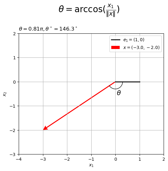
2次元ベクトルと標準単位ベクトルのなす角を円弧(角マーク)で示すグラフを作成する。
なす角については「【Python】3.4:ベクトルとx軸のなす角の可視化【『スタンフォード線形代数入門』のノート】 - からっぽのしょこ」を参照のこと。
2次元ベクトル を作成して、なす角を計算する。
# 2次元ベクトルを指定
x = np.array([-3.0, -2.0])

# ベクトルxとx軸のなす角(ラジアン)を計算
theta = np.arccos(x[0] / np.linalg.norm(x))
print(theta) # 0からπの値
print(theta / np.pi) # 0から1の値
2.5535900500422257
0.8128329581890013
ベクトル を1次元配列
x として値を指定する。Pythonではインデックスが0から割り当てられるので、 は
x[0] に対応することに注意する。
と標準単位ベクトル
のなす角
は、次の式で計算できる。
はラジアン(弧度法における角度)であり、
の値(度数法による角度
に対応)をとる。ただし、
が0ベクトルだと0除算になるため定義できない(計算結果が
nan になる)。
コサイン関数 の逆関数(逆コサイン関数)
は
np.arccos()、ユークリッドノルム は
np.linalg.norm() で計算できる。
2つのベクトル(線分)によって、劣角 と優角
の2つの角(度数法だと劣角
と優角
)ができる。
なす角 は劣角の角度に対応する。
作図用の角度を計算する。
# 座標に応じて符号を変換
sgn_x   = 1.0 if x[1] >= 0.0 else -1.0
theta_x = sgn_x * theta
print(theta_x)
-2.5535900500422257
作図用のなす角を で表すことにする。
x軸線の正の部分(標準単位ベクトル)から左回りにできる角が優角のとき、言い換えると、 が負の値(ベクトル
が第3・4象限)のとき、右回りにできる劣角を負の角度
として扱う。
が0以上の値(ベクトル
が第1・2象限)のとき、
を用いる。
ベクトル x のy軸の値 x[1] が、0 以上であれば sgn_x を正の符号 1、0 未満であれば負の符号 -1 にする。
y座標の符号となす角の積を theta_x とする。
角マークと角ラベルの座標を計算する。
# 角マーク用のラジアンを作成
t_vals = np.linspace(start=0.0, stop=sgn_x * theta, num=100)
print(t_vals[:5])

# 角マークの座標を計算
r = 0.3
angle_mark_arr = np.vstack(
    [r * np.cos(t_vals),
     r * np.sin(t_vals)]
)
print(angle_mark_arr[:, :5])

# 角ラベルの座標を計算
r = 0.5
angle_label_vec = np.array(
    [r * np.cos(0.5 * theta_x),
     r * np.sin(0.5 * theta_x)]
)
print(angle_label_vec)
[ 0.         -0.02579384 -0.05158768 -0.07738152 -0.10317536]
[[ 0.3         0.29990021  0.2996009   0.29910226  0.29840464]
 [ 0.         -0.00773729 -0.01546944 -0.02319129 -0.03089772]]
[ 0.14489207 -0.47854601]
から
までのラジアン
を作成して、角マークの座標を計算する。
角マークは、半径を として、次の式で円弧の座標(x軸・y軸の値)
を計算する。
半径 r で角マークのサイズ(原点からのノルム)を調整する。
角ラベルは、円弧(なす角)の中点に配置するため、ノルムを として、次の式で座標を計算する。
ノルム r で角ラベルの位置(原点からのノルム)を調整する。
2次元空間上にベクトル となす角のグラフを作成する。
# グラフサイズを設定
x_min = np.floor(np.min([0.0, x[0]])) - 1
x_max =  np.ceil(np.max([1.0, x[0]])) + 1
y_min = np.floor(np.min([0.0, x[1]])) - 1
y_max =  np.ceil(np.max([1.0, x[1]])) + 1

# 2Dベクトルのなす角を作図
fig, ax = plt.subplots(figsize=(6, 6), facecolor='white')
ax.plot([0, 1], [0, 0],
        color='black', linewidth=2,
        label='$e_1 = (1, 0)$') # 標準単位ベクトルe1
ax.quiver(0, 0, *x,
          color='red', units='dots', width=3, headwidth=5,
          angles='xy', scale_units='xy', scale=1,
          label='$x = ({}, {})$'.format(*x)) # ベクトルx
ax.plot(*angle_mark_arr,
        color='black', linewidth=1) # 角マーク
ax.text(*angle_label_vec,
        s='$\\theta$', size=15, ha='center', va='center') # 角ラベル
ax.set_xticks(ticks=np.arange(x_min, x_max+1))
ax.set_yticks(ticks=np.arange(y_min, y_max+1))
ax.set_xlabel('$x_1$')
ax.set_ylabel('$x_2$')
ax.set_title('$\\theta = {:.2f}'.format(theta / np.pi)+'\pi, ' +
             '\\theta^\circ = {:.1f}'.format(theta * 180.0/np.pi)+'^\circ$', loc='left')
fig.suptitle('$\\theta = \\arccos(\\frac{x_1}{\|x\|})$', fontsize=20)
ax.grid()
ax.legend()
ax.set_aspect('equal')
plt.show()
plt.quiver() でベクトルを描画する。第1・2引数に始点(原点)の座標、第3・4引数に移動量(ベクトル)を指定する。
配列 x の頭に * を付けてアンパック(展開)して指定している。
標準単位ベクトル を
plt.plot() で描画する。第1引数に始点と終点のx軸座標、第2引数にy軸座標を指定する。
ベクトルの値を変化させたアニメーションを作成する。
・作図コード(クリックで展開)
# フレーム数を指定
frame_num = 60

# 変化するベクトルを作成
beta = 1.5
rad_n = np.linspace(start=0.0, stop=2.0*np.pi, num=frame_num+1)[:frame_num]
x_n = np.array(
    [beta * np.cos(rad_n), beta * np.sin(rad_n)]
).T

# グラフサイズを設定
x_min = np.floor(np.min([0.0, *x_n[:, 0]]))
x_max =  np.ceil(np.max([1.0, *x_n[:, 0]]))
y_min = np.floor(np.min([0.0, *x_n[:, 1]]))
y_max =  np.ceil(np.max([1.0, *x_n[:, 1]]))

# グラフオブジェクトを初期化
fig, ax = plt.subplots(figsize=(6, 6), facecolor='white')
fig.suptitle('$\\theta = \\arccos(\\frac{x_1}{\|x\|})$', fontsize=20)

# 作図処理を関数として定義
def update(i):

    # 前フレームのグラフを初期化
    plt.cla()

    # i番目のベクトルを取得
    x = x_n[i]

    # ベクトルxとx軸のなす角(ラジアン)を計算
    theta = np.arccos(x[0] / np.linalg.norm(x))

    # 座標に応じて符号を変換
    sgn_x   = 1.0 if x[1] >= 0.0 else -1.0
    theta_x = sgn_x * theta

    # 角マーク用のラジアンを作成
    t_vals = np.linspace(start=0.0, stop=theta_x, num=100)

    # 角マークの座標を計算
    r = 0.3
    angle_mark_arr = np.vstack(
        [r * np.cos(t_vals),
         r * np.sin(t_vals)]
    )

    # 角ラベルの座標を計算
    r = 0.45
    angle_label_vec = np.array(
        [r * np.cos(0.5 * theta_x),
         r * np.sin(0.5 * theta_x)]
    )

    # 2Dベクトルのなす角を作図
    ax.plot([0, 1], [0, 0],
            color='black', linewidth=2,
            label='$e_1 = (1, 0)$') # 標準単位ベクトルe1
    ax.quiver(0, 0, *x,
              color='red', units='dots', width=3, headwidth=5,
              angles='xy', scale_units='xy', scale=1,
              label='$x = ({: .2f}, {: .2f})$'.format(*x)) # ベクトルx
    ax.plot(*angle_mark_arr,
            color='black', linewidth=1) # 角マーク
    ax.text(*angle_label_vec,
            s='$\\theta$', size=15, ha='center', va='center') # 角ラベル
    ax.set_xticks(ticks=np.arange(x_min, x_max+1))
    ax.set_yticks(ticks=np.arange(y_min, y_max+1))
    ax.set_xlabel('$x_1$')
    ax.set_ylabel('$x_2$')
    ax.set_title('$\\theta = {:.2f}'.format(theta / np.pi)+'\pi, ' +
                 '\\theta^\circ = {:.1f}'.format(theta * 180.0/np.pi)+'^\circ$', loc='left')
    ax.grid()
    ax.legend(loc='upper left')
    ax.set_aspect('equal')

# gif画像を作成
ani = FuncAnimation(fig=fig, func=update, frames=frame_num, interval=100)

# gif画像を保存
ani.save(filename='2d_angle_x.gif')
作図処理をupdate()として定義して、FuncAnimation()でgif画像を作成します。

円弧の描画
2次元ベクトルとx軸線を繋ぐ円弧(角マーク)の座標計算とノルム操作をグラフで確認する。
2次元ベクトル を作成して、ノルムを計算する。
# 2次元ベクトルを指定
x = np.array([-3.0, -2.0])

# ノルムを計算
norm_x = np.linalg.norm(x)
print(norm_x)
3.605551275463989
ベクトル を1次元配列
x として値を指定する。
次元ベクトル
のユークリッドノルム
を np.linalg.norm() で計算する。
x軸方向の標準単位ベクトルを とする。標準単位ベクトルのノルムは次元に関わらず
である。
ベクトル をグラフで確認する。
# グラフサイズを設定
x_min = np.floor(np.min([0.0, x[0]])) - 1
x_max =  np.ceil(np.max([1.0, x[0]])) + 1
y_min = np.floor(np.min([0.0, x[1]])) - 1
y_max =  np.ceil(np.max([1.0, x[1]])) + 1

# 2Dベクトルを作図
fig, ax = plt.subplots(figsize=(6, 6), facecolor='white')
ax.scatter(0, 0,
           color='orange', s=100, label='$O = (0, 0)$') # 原点
ax.scatter(1, 0,
           color='black', s=100, label='$e_1 = (1, 0)$') # x軸線上の点
ax.scatter(*x,
           color='red', s=100, label='$x = ({}, {})$'.format(*x)) # 点x
ax.plot([0, 1], [0, 0],
        color='black', linewidth=2) # 標準単位ベクトルe1
ax.quiver(0, 0, *x,
          color='red', units='dots', width=3, headwidth=5,
          angles='xy', scale_units='xy', scale=1) # ベクトルx
ax.set_xticks(ticks=np.arange(x_min, x_max+1))
ax.set_yticks(ticks=np.arange(y_min, y_max+1))
ax.set_xlabel('$x_1$')
ax.set_ylabel('$x_2$')
ax.set_title('$\|e_1\| = {}, \|x\| = {:.2f}$'.format(np.linalg.norm([1, 0]), norm_x), loc='left')
fig.suptitle('$x = (x_1, x_2)$', fontsize=20)
ax.grid()
ax.legend()
ax.set_aspect('equal')
plt.show()
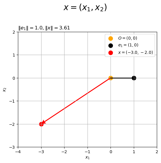
ベクトル のノルム
は、原点
と点
の距離に対応する。
ここから、円周上の2点を考える。
半径を指定して、円周の座標を計算する。
# 半径(ノルム)を指定
r = 2.5

# 円周用のラジアンを作成
t_vals = np.linspace(start=0.0, stop=2.0*np.pi, num=100)
print(t_vals[:5])

# 円周の座標を計算
circle_x_vals = r * np.cos(t_vals)
circle_y_vals = r * np.sin(t_vals)
print(circle_x_vals[:5])
print(circle_y_vals[:5])
print(np.linalg.norm(np.vstack([circle_x_vals[:5], circle_y_vals[:5]]), axis=0))
[0.         0.06346652 0.12693304 0.19039955 0.25386607]
[2.5        2.49496669 2.47988703 2.45482174 2.41987175]
[0.         0.1585598  0.31648113 0.47312811 0.62786997]
[2.5 2.5 2.5 2.5 2.5]
原点を中心とする円周の座標 は、半径を
として、
から
までのラジアン
を用いて、次の式で計算できる。
circle_*_vals の同じインデックスの要素が、円周上の各点の座標に対応する。
円周上の点のノルム(中心との距離)は半径 になる。
ベクトルのノルムを変更する。
# ベクトルのノルムを調整
tilde_x = r * x / np.linalg.norm(x)
print(tilde_x)
print(np.linalg.norm(tilde_x))
[-2.08012574 -1.38675049]
2.5000000000000004
をノルムで割るとノルムが1のベクトルになり、さらに
を掛けるとノルムが
のベクトルになる。
ベクトル (の延長線)と円周の交点
をグラフで確認する。
# グラフサイズを設定
x_min = np.floor(np.min([-r, x[0]])) - 1
x_max =  np.ceil(np.max([r, x[0]])) + 1
y_min = np.floor(np.min([-r, x[1]])) - 1
y_max =  np.ceil(np.max([r, x[1]])) + 1

# 2Dベクトルを結ぶ円周を作図
fig, ax = plt.subplots(figsize=(6, 6), facecolor='white')
ax.plot(circle_x_vals, circle_y_vals,
        color='black', linewidth=1.5) # 円周
ax.scatter(0, 0,
           color='orange', s=100, label='$O = (0, 0)$') # 原点
ax.scatter(r, 0,
           color='black', s=100, label='$r\ e_1 = ('+str(r)+', 0)$') # x軸線上の点
ax.scatter(*tilde_x,
           color='red', s=100,
           label='$\\tilde{x} = [tex: '+'$({:.2f}, {:.2f})$'.format(*tilde_x)) # 点x
ax.plot([0, r], [0, 0],
        color='black', linewidth=2) # x軸線
ax.quiver(0, 0, *x,
          color='red', units='dots', width=3, headwidth=5,
          angles='xy', scale_units='xy', scale=1) # ベクトルx
if norm_x < r:
    ax.plot([x[0], tilde_x[0]], [x[1], tilde_x[1]],
            color='red', linewidth=2, linestyle=':') # ベクトルxの延長線
ax.set_xticks(ticks=np.arange(x_min, x_max+1))
ax.set_yticks(ticks=np.arange(y_min, y_max+1))
ax.set_xlabel('$x_1$')
ax.set_ylabel('$x_2$')
ax.set_title('$r = '+str(r)+', ' +
             '\|\\tilde{x}\| = '+'{:.2f}$'.format(np.linalg.norm(tilde_x)), loc='left')
fig.suptitle('$\\tilde{x} = r \\frac{x}{\|x\|}$', fontsize=20)
ax.grid()
ax.legend(loc='upper right')
ax.set_aspect('equal')
plt.show()
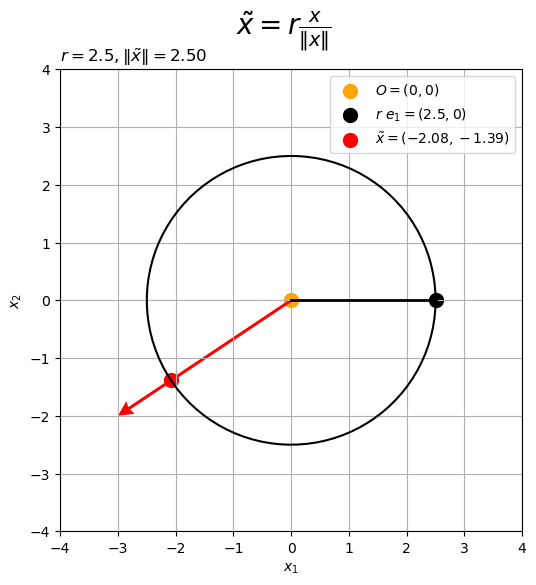
「半径 の円周」は中心からの距離が
の点の集合なので、「ノルムが
のベクトル
」は円周上の点であり、円周とベクトル
(の延長線)の交点になる。
円周上の2点が得られた。続いて、2点を結ぶ円弧を考える。
ベクトル のなす角を計算する。
# ベクトルxとx軸のなす角(ラジアン)を計算
theta = np.arccos(x[0] / norm_x)
print(theta)

# 円周上の点を作成
p = np.array(
    [r * np.cos(theta), r * np.sin(theta)]
)
print(p)
print(np.linalg.norm(p))
2.5535900500422257
[-2.08012574  1.38675049]
2.5
のなす角
は、次の式で計算できる。
ラジアン を用いて、円周上の点
の座標を計算する。
円周の座標と同様に、ノルムは半径になる。
となす角
の関係をグラフで確認する。
# ラベル位置の調整値を指定
d = 1.2

# x軸の値を計算
c1 = r * np.cos(theta)

# 2Dベクトルを結ぶ円周を作図
fig, ax = plt.subplots(figsize=(6, 6), facecolor='white')
ax.plot(circle_x_vals, circle_y_vals,
        color='black', linewidth=1.5) # 円周
ax.scatter(r, 0,
           color='black', s=100, label='$r\ e_1 = (r, 0)$') # x軸線上の点
ax.scatter(c1, 0,
           facecolor='white', edgecolor='blue', s=100, linestyle='--',
           label='$(r\ \cos \\theta, 0)$') # 点cosθ
ax.scatter(*p,
           facecolor='white', edgecolor='red', s=100, linestyle='--',
           label='$p = ({:.2f}, {:.2f})$'.format(*p)) # 点p
ax.scatter(*tilde_x,
           color='red', s=100,
           label='$\\tilde{x} = [tex: '+'$({:.2f}, {:.2f})$'.format(*tilde_x)) # 点x
ax.plot([0, r], [0, 0],
        color='black', linewidth=2) # x軸線
ax.plot([0, c1], [0, 0],
        color='blue', linewidth=1.5, linestyle='--') # 補助線cosθ
ax.plot([c1, tilde_x[0]], [0, tilde_x[1]],
        color='black', linewidth=1.5, linestyle=':') # 補助線x
if x[1] < 0.0:
    ax.plot([c1, p[0]], [0, p[1]],
            color='black', linewidth=1.5, linestyle=':') # 補助線p
    ax.plot([0, p[0]], [0, p[1]],
            color='red', linewidth=2, linestyle='--') # ベクトルp
    ax.text(*d*tilde_x,
            s='$- \\theta$', size=15, ha='center', va='center') # ラジアンラベルx
ax.quiver(0, 0, *x,
          color='red', units='dots', width=3, headwidth=5,
          angles='xy', scale_units='xy', scale=1) # ベクトルx
if norm_x < r:
    ax.plot([x[0], tilde_x[0]], [x[1], tilde_x[1]],
            color='red', linewidth=2, linestyle=':') # ベクトルxの延長線
ax.text(*d*p,
        s='$\\theta$', size=15, ha='center', va='center') # ラジアンラベルp
ax.text(d*r, 0,
        s='$0$', size=15, ha='center', va='center') # ラジアンラベルe1
ax.set_xticks(ticks=np.arange(x_min, x_max+1))
ax.set_yticks(ticks=np.arange(y_min, y_max+1))
ax.set_xlabel('$x_1$')
ax.set_ylabel('$x_2$')
ax.set_title('$r = {}, \\theta = {:.2f} \pi$'.format(r, theta/np.pi), loc='left')
fig.suptitle('$\\theta = \\arccos(\\frac{x_1}{\|x\|})$', fontsize=20)
ax.grid()
ax.legend(loc='upper right')
ax.set_aspect('equal')
plt.show()
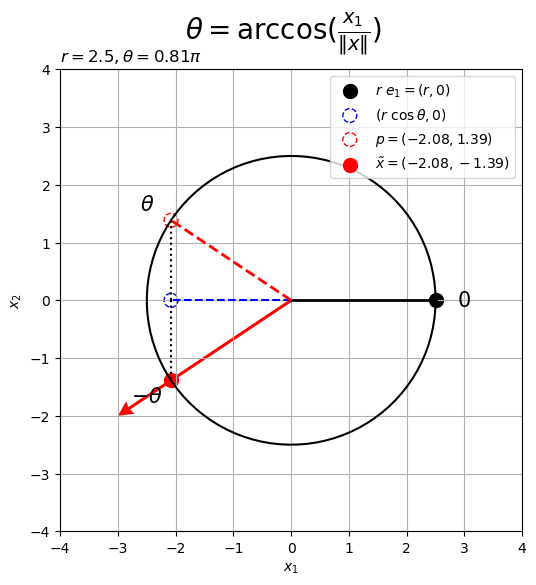
x軸線の正の部分から左回りに 移動した点の座標は
である。
なす角は なので、
のy軸の値が正
のとき
、負
のとき
となる。
ベクトルの座標によって、 の移動方向(右回り・左回り)が変わる。
座標に応じて、円弧の座標を計算する。
# 円弧用のラジアンを作成
if x[1] >= 0.0:
    u_vals = np.linspace(start=0.0, stop=theta, num=100)
else:
    u_vals = np.linspace(start=-theta, stop=0.0, num=100)
print(u_vals[:5])

# 円弧の座標を計算
arc_x_vals = r * np.cos(u_vals)
arc_y_vals = r * np.sin(u_vals)
print(arc_x_vals[:5])
print(arc_y_vals[:5])
print(np.linalg.norm(np.vstack([arc_x_vals[:5], arc_y_vals[:5]]), axis=0))
[-2.55359005 -2.52779621 -2.50200237 -2.47620853 -2.45041469]
[-2.08012574 -2.04366814 -2.00585093 -1.96669926 -1.92623916]
[-1.38675049 -1.43993768 -1.49216689 -1.54340339 -1.59361309]
[2.5 2.5 2.5 2.5 2.5]
原点を中心とする半径が の円弧の座標
は、
のy軸座標が「正
のとき
から
まで」、「負
のとき
から
まで」のラジアン
を用いて、次の式で計算できる。
円周の座標と同様に、ノルムは半径になる。
点 を結ぶ半径
の円弧を描画する。
# y座標の符号を取得
sgn_y = 1.0 if x[1] >= 0.0 else -1.0

# 2Dベクトルを結ぶ円弧を作図
fig, ax = plt.subplots(figsize=(6, 6), facecolor='white')
ax.plot(circle_x_vals, circle_y_vals,
        color='black', linewidth=1.5, linestyle=':') # 円周
ax.plot(arc_x_vals, arc_y_vals,
        color='black', linewidth=2) # 円弧
ax.scatter(r, 0,
           color='black', s=100, label='$r\ e_1 = (r, 0)$') # x軸線上の点
ax.scatter(*tilde_x,
           color='red', s=100,
           label='$\\tilde{x} = [tex: '+'$({:.2f}, {:.2f})$'.format(*tilde_x)) # 点x
ax.plot([0, r], [0, 0],
        color='black', linewidth=2) # x軸線
ax.quiver(0, 0, *x,
          color='red', units='dots', width=3, headwidth=5,
          angles='xy', scale_units='xy', scale=1) # ベクトルx
if norm_x < r:
    ax.plot([x[0], tilde_x[0]], [x[1], tilde_x[1]],
            color='red', linewidth=2, linestyle=':') # ベクトルxの延長線
ax.text(d*r, 0,
        s='$0$', size=15, ha='center', va='center') # ラジアンラベルe1
ax.text(*d*tilde_x,
        s='$\\theta$', size=15, ha='center', va='center') # なす角ラベル
ax.set_xticks(ticks=np.arange(x_min, x_max+1))
ax.set_yticks(ticks=np.arange(y_min, y_max+1))
ax.set_xlabel('$x_1$')
ax.set_ylabel('$x_2$')
ax.set_title('$x = ({}, {}), r = {}'.format(*x, r)+', ' +
             '\\theta = {:.2f} \pi$'.format(sgn_y*theta/np.pi), loc='left')
fig.suptitle('$\\theta = \mathrm{sgn(x_2)} \\arccos(\\frac{x_1}{\|x\|})$', fontsize=20)
ax.grid()
ax.legend()
ax.set_aspect('equal')
plt.show()
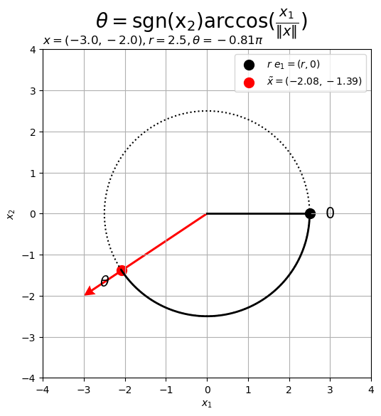
変数 の符号を返す関数を
とする(正確には符号関数は0のとき0になるが、この例では0のとき正の値とする)。
円座標 は、符号関数を用いて、次の式で求められる。
詳しくは、極座標系を参照のこと。
以上で、円周上の2点を結ぶ円弧が得られた。
ベクトルの値を変化させたアニメーションを作成する。
・作図コード(クリックで展開)
# フレーム数を指定
frame_num = 60

# 変化するベクトルを作成
beta = 4.0
rad_n = np.linspace(start=0.0, stop=2.0*np.pi, num=frame_num+1)[:frame_num]
x_n = np.array(
    [beta * np.cos(rad_n), beta * np.sin(rad_n)]
).T

# 半径を指定
r = 2.5

# 円周の座標を計算
t_vals = np.linspace(start=0.0, stop=2.0*np.pi, num=100)
circle_x_vals = r * np.cos(t_vals)
circle_y_vals = r * np.sin(t_vals)

# グラフサイズを設定
axis_size = np.ceil(np.max([r, abs(beta)])) + 1

# グラフオブジェクトを初期化
fig, ax = plt.subplots(figsize=(6, 6), facecolor='white')
fig.suptitle('$\\theta = \\arccos(\\frac{x_1}{\|x\|})$', fontsize=20)

# 作図処理を関数として定義
def update(i):

    # 前フレームのグラフを初期化
    plt.cla()

    # i番目のベクトルを取得
    x = x_n[i]

    # ノルムを調整
    tilde_x = r * x / np.linalg.norm(x)

    # ベクトルxとx軸のなす角(ラジアン)を計算
    theta = np.arccos(x[0] / np.linalg.norm(x))

    # 円周上の点を作成
    p = np.array([r * np.cos(theta), r * np.sin(theta)])

    # 円弧の座標を計算
    theta_x = theta if x[1] >= 0.0 else -theta
    u_vals = np.linspace(start=0.0, stop=theta_x, num=100)
    arc_x_vals = r * np.cos(u_vals)
    arc_y_vals = r * np.sin(u_vals)

    # 2Dベクトルを結ぶ円弧を作図
    d = 1.2
    ax.plot(circle_x_vals, circle_y_vals,
            color='black', linewidth=1.5, linestyle=':') # 円周
    ax.plot(arc_x_vals, arc_y_vals,
            color='black', linewidth=2) # 円弧
    ax.scatter(r, 0,
               color='black', s=100, label='$r\ e_1 = (r, 0)$') # x軸線上の点
    ax.scatter(*p,
               facecolor='white', edgecolor='red', s=100, linestyle='--',
               label='$p = ({: .2f}, {: .2f})$'.format(*p)) # 点p
    ax.scatter(*tilde_x,
               color='red', s=100,
               label='$\\tilde{x} = [tex: '+'$({: .2f}, {: .2f})$'.format(*tilde_x)) # 点x
    ax.plot([0, r], [0, 0],
            color='black', linewidth=2) # x軸線
    if x[1] < 0.0:
        ax.plot([tilde_x[0], p[0]], [tilde_x[1], p[1]],
                color='black', linewidth=1.5, linestyle=':') # 補助線xp
        ax.plot([0, p[0]], [0, p[1]],
                color='red', linewidth=2, linestyle='--') # ベクトルp
        ax.text(*d*tilde_x,
                s='$- \\theta$', size=15, ha='center', va='center') # ラジアンラベルx
    ax.quiver(0, 0, *x,
              color='red', units='dots', width=3, headwidth=5,
              angles='xy', scale_units='xy', scale=1) # ベクトルx
    if np.linalg.norm(x) < r:
        ax.plot([x[0], tilde_x[0]], [x[1], tilde_x[1]],
                color='red', linewidth=2, linestyle=':') # ベクトルxの延長線
    ax.text(*d*p,
            s='$\\theta$', size=15, ha='center', va='center') # ラジアンラベルp
    ax.text(d*r, 0,
            s='$0$', size=15, ha='center', va='center') # ラジアンラベルe1
    ax.set_xticks(ticks=np.arange(-axis_size, axis_size+1))
    ax.set_yticks(ticks=np.arange(-axis_size, axis_size+1))
    ax.set_xlabel('$x_1$')
    ax.set_ylabel('$x_2$')
    ax.set_title('$x = ({: .2f}, {: .2f})'.format(*x)+', ' +
                 'r = {}'+str(r)+', ' +
                 '\\theta = {:.2f} \pi'.format(theta/np.pi)+'$', loc='left')
    fig.suptitle('$\\theta = \\arccos(\\frac{x_1}{\|x\|})$', fontsize=20)
    ax.grid()
    ax.legend(loc='upper left')
    ax.set_aspect('equal')

# gif画像を作成
ani = FuncAnimation(fig=fig, func=update, frames=frame_num, interval=100)

# gif画像を保存
ani.save(filename='2d_arc_x.gif')
ベクトル のy座標の符号(正負)によって円弧を描画する向きが変わるのが分かる。
この記事では、2次元空間における1つの線分を結ぶ曲線を扱った。次の記事では、2つの線分を結ぶ曲線を扱う。
おわりに
なんとも解説するのが面倒で書きかけで放置してしまってました。たしかスタンフォード線形代数シリーズの5章の補足として書き始めたのですが、放置したまま6章が書き終わりました。原型は3章の時点で書けてたはずなのに。放置したままでずっと気持ち悪かったので、いいかげん書き切ろう再開しましたがやっぱり筆が重かったです。
なんでこんなに説明が大変なんだって、1つの記事に内容を詰め込みすぎなんだと気付きました。説明の説明をすると、話が入り組むし構成がややこしくなるのも当然ですね。というわけで、書きたかったメインの内容は次の記事で、この記事はその内容を説明するための説明で、そもそもが本筋の説明でもあるみたいな感じです。この説明だけでもうメンドいね。
他の記事との統一感と1記事での読み応えとか、検索のされやすさと管理のしやすさとか、記事の粒度って意外と難しくてずっと悩んでます。この記事も2つの内容を書いてる気がします。
2023年8月4日は、こぶしファクトリーの元リーダーの広瀬彩海さんの24歳お誕生です。
こぶしの曲も最高なのでぜひ聴いてください。
【次の内容】