はじめに
調べても分からなかったので自分なりにやってみる黒魔術シリーズです。もっといい方法があれば教えてください。
この記事では、円周上の2点をいい感じに繋ぐ曲線のグラフを作成します。
【前の内容】
【目次】
円周上の2点を結ぶ円弧を作図したい
Matplotlibライブラリを利用して、2次元空間における円周(circle)上の2点を結ぶ良い感じの曲線を作成したい。また、その円弧(circular arc)の半径を調整して、2つの2次元ベクトルのなす角(angle between two vectors)を示したい。
度数法と弧度法の角度の関係や、角度と座標の関係については「円周の作図【Matplotlib】 - からっぽのしょこ」を参照のこと。
利用するライブラリを読み込みます。
# 利用ライブラリ
import numpy as np
import matplotlib.pyplot as plt
from matplotlib.animation import FuncAnimation
なす角の描画
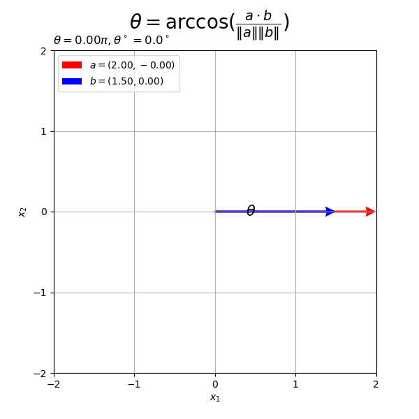
まずは、完成図(やりたいこと)を確認する。
2つの2次元ベクトルのなす角を円弧(角マーク)で示すグラフを作成する。
なす角については「【Python】3.4:2つのベクトルのなす角の可視化【『スタンフォード線形代数入門』のノート】 - からっぽのしょこ」を参照のこと。
2次元ベクトル を作成して、なす角を計算する。
# 2次元ベクトルを指定
a = np.array([2.0, 1.0])
b = np.array([-2.0, -2.0])

# ベクトルa,bのなす角(ラジアン)を計算
cos_theta = np.dot(a, b) / np.linalg.norm(a) / np.linalg.norm(b)
theta = np.arccos(cos_theta)
print(theta) # 0からπの値
print(theta / np.pi) # 0から1の値
2.819842099193151
0.8975836176504333
2つのベクトル を1次元配列
a, b として値を指定する。Pythonではインデックスが0から割り当てられるので、 は
a[0] に対応することに注意する。
のなす角
は、次の式で計算できる。
はラジアン(弧度法における角度)であり、
の値(度数法による角度
に対応)をとる。ただし、
または
が0ベクトルだと0除算になるため定義できない(計算結果が
nan になる)。
コサイン関数 の逆関数(逆コサイン関数)
は
np.arccos()、内積 は
np.dot()、ユークリッドノルム は
np.linalg.norm() で計算できる。
2つのベクトル(線分)によって、劣角 と優角
の2つの角(度数法だと劣角
と優角
)ができる。
なす角 は劣角の角度に対応する。
それぞれのなす角を計算する。
# ベクトルaとx軸のなす角(ラジアン)を計算
sgn_a   = 1.0 if a[1] >= 0.0 else -1.0
theta_a = sgn_a * np.arccos(a[0] / np.linalg.norm(a))
print(theta_a / np.pi)

# ベクトルbとx軸のなす角(ラジアン)を計算
sgn_b   = 1.0 if b[1] >= 0.0 else -1.0
theta_b = sgn_b * np.arccos(b[0] / np.linalg.norm(b))
print(theta_b / np.pi)

# 角度の差に応じて負の角度を優角に変換
if abs(theta_a - theta_b) > np.pi:
    theta_a = theta_a if a[1] >= 0.0 else theta_a + 2.0*np.pi
    theta_b = theta_b if b[1] >= 0.0 else theta_b + 2.0*np.pi
print(theta_a / np.pi)
print(theta_b / np.pi)
0.1475836176504333
-0.75
0.1475836176504333
-0.75
ベクトル それぞれと標準単位ベクトル(x軸の正の部分)
のなす角を
で表し、次の式で計算する。
x軸線の正の部分から左回りにできる角が優角のとき( が負の値のとき)、右回りにできる劣角を負の角度
として扱う。
この操作を、符号関数 を用いて数式で表している(正確には符号関数は0のとき0になるが、この例では0のとき正の値とする)。
詳しくは「【Python】円周上の点とx軸を結ぶ円弧を作図したい - からっぽのしょこ」を参照のこと。
ただし、 の差が優角になる場合(一方が正の角度でもう一方が負の角度で、差の絶対値
が
を超える場合)は、負の角度の方に
を足して優角に変換する。
角マークと角ラベルの座標を計算する。
# 角マーク用のラジアンを作成
t_vals = np.linspace(start=theta_a, stop=theta_b, num=100)
print(t_vals[:5])

# 角マークの座標を計算
r = 0.3
angle_mark_arr = np.vstack(
    [r * np.cos(t_vals),
     r * np.sin(t_vals)]
)
print(angle_mark_arr[:5, :5])

# 角ラベルの座標を計算
r = 0.5
angle_label_vec = np.array(
    [r * np.cos(np.median(t_vals)),
     r * np.sin(np.median(t_vals))]
)
print(angle_label_vec)
[0.46364761 0.43516436 0.4066811  0.37819785 0.34971459]
[[0.26832816 0.27204023 0.27553161 0.27879947 0.28184116]
 [0.13416408 0.12646783 0.11866899 0.11077388 0.10278891]]
[ 0.29235514 -0.40562109]
から
までのラジアン
を作成して、角マークと角ラベルの座標を計算する。
角マークは、半径を として、次の式で円弧の座標(x軸・y軸の値)
を計算する。
半径 r で角マークのサイズ(原点からのノルム)を調整する。
角ラベルは、円弧(なす角)の中点に配置する。
r で角ラベルの位置(原点からのノルム)を調整する。
2次元空間上にベクトル となす角のグラフを作成する。
# グラフサイズを設定
x_min = np.floor(np.min([0.0, a[0], b[0]])) - 1
x_max =  np.ceil(np.max([0.0, a[0], b[0]])) + 1
y_min = np.floor(np.min([0.0, a[1], b[1]])) - 1
y_max =  np.ceil(np.max([0.0, a[1], b[1]])) + 1

# 2Dベクトルのなす角を作図
fig, ax = plt.subplots(figsize=(6, 6), facecolor='white')
ax.quiver(0, 0, *a,
          color='red', units='dots', width=3, headwidth=5,
          angles='xy', scale_units='xy', scale=1,
          label='$a = ({}, {}'.format(*a)+')$') # ベクトルa
ax.quiver(0, 0, *b,
          color='blue', units='dots', width=3, headwidth=5,
          angles='xy', scale_units='xy', scale=1,
          label='$b =({}, {}'.format(*b)+')$') # ベクトルb
ax.plot(*angle_mark_arr,
        color='black', linewidth=1) # 角マーク
ax.text(*angle_label_vec,
        s='$\\theta$', size=15, ha='center', va='center') # 角ラベル
ax.set_xticks(ticks=np.arange(x_min, x_max+1))
ax.set_yticks(ticks=np.arange(y_min, y_max+1))
ax.set_xlabel('$x_1$')
ax.set_ylabel('$x_2$')
ax.set_title('$\\theta = {:.2f}'.format(theta / np.pi)+'\pi, ' +
             '\\theta^\circ = {:.1f}'.format(theta * 180.0/np.pi)+'^\circ$', loc='left')
fig.suptitle('$\\theta = \\arccos(\\frac{a \cdot b}{\|a\| \|b\|})$', fontsize=20)
ax.grid()
ax.legend()
ax.set_aspect('equal')
plt.show()

plt.quiver() でベクトルを描画する。第1・2引数に始点(原点)の座標、第3・4引数に移動量(ベクトル)を指定する。
配列 x の頭に * を付けてアンパック(展開)して指定している。
ベクトルの値を変化させたアニメーションを作成する。
・作図コード(クリックで展開)
# フレーム数を指定
frame_num = 60

# 変化するベクトルを作成
alpha, beta = 2.0, 1.5
rad_n = np.linspace(start=0.0, stop=2.0*np.pi, num=frame_num+1)[:frame_num]
a_n = np.array(
    [alpha * np.cos(-2.0 * rad_n), alpha * np.sin(-2.0 * rad_n)]
).T
b_n = np.array(
    [beta * np.cos(rad_n), beta * np.sin(rad_n)]
).T

# グラフサイズを設定
x_min = np.floor(np.min([0.0, *a_n[:, 0], *b_n[:, 0]]))
x_max =  np.ceil(np.max([1.0, *a_n[:, 0], *b_n[:, 0]]))
y_min = np.floor(np.min([0.0, *a_n[:, 1], *b_n[:, 1]]))
y_max =  np.ceil(np.max([1.0, *a_n[:, 1], *b_n[:, 1]]))

# グラフオブジェクトを初期化
fig, ax = plt.subplots(figsize=(6, 6), facecolor='white')
fig.suptitle('$\\theta = \\arccos(\\frac{a \cdot b}{\|a\| \|b\|})$', fontsize=20)

# 作図処理を関数として定義
def update(i):

    # 前フレームのグラフを初期化
    plt.cla()

    # i番目のベクトルを取得
    a = a_n[i]
    b = b_n[i]

    # ベクトルa,bのなす角(ラジアン)を計算
    theta = np.arccos(
        np.dot(a, b) / np.linalg.norm(a) / np.linalg.norm(b)
    )

    # ベクトルa・bとx軸のなす角(ラジアン)を計算
    sgn_a   = 1.0 if a[1] >= 0.0 else -1.0
    theta_a = sgn_a * np.arccos(a[0] / np.linalg.norm(a))
    sgn_b   = 1.0 if b[1] >= 0.0 else -1.0
    theta_b = sgn_b * np.arccos(b[0] / np.linalg.norm(b))

    # 角度の差に応じて負の角度を優角に変換
    if abs(theta_a - theta_b) > np.pi:
        theta_a = theta_a if a[1] >= 0.0 else theta_a + 2.0*np.pi
        theta_b = theta_b if b[1] >= 0.0 else theta_b + 2.0*np.pi

    # 角マーク用のラジアンを作成
    t_vals = np.linspace(start=theta_a, stop=theta_b, num=100)

    # 角マークの座標を計算
    r = 0.3
    angle_mark_arr = np.vstack(
        [r * np.cos(t_vals),
         r * np.sin(t_vals)]
    )

    # 角ラベルの座標を計算
    r = 0.45
    angle_label_vec = np.array(
        [r * np.cos(np.median(t_vals)),
         r * np.sin(np.median(t_vals))]
    )

    # 2Dベクトルのなす角を作図
    ax.quiver(0, 0, *a,
              color='red', units='dots', width=3, headwidth=5,
              angles='xy', scale_units='xy', scale=1,
              label='$a = ({: .2f}, {: .2f}'.format(*a)+')$') # ベクトルa
    ax.quiver(0, 0, *b,
              color='blue', units='dots', width=3, headwidth=5,
              angles='xy', scale_units='xy', scale=1,
              label='$b =({: .2f}, {: .2f}'.format(*b)+')$') # ベクトルb
    ax.plot(*angle_mark_arr,
            color='black', linewidth=1) # 角マーク
    ax.text(*angle_label_vec,
            s='$\\theta$', size=15, ha='center', va='center') # 角ラベル
    ax.set_xticks(ticks=np.arange(x_min, x_max+1))
    ax.set_yticks(ticks=np.arange(y_min, y_max+1))
    ax.set_xlabel('$x_1$')
    ax.set_ylabel('$x_2$')
    ax.set_title('$\\theta = {:.2f}'.format(theta / np.pi)+'\pi, ' +
                 '\\theta^\circ = {:.1f}'.format(theta * 180.0/np.pi)+'^\circ$', loc='left')
    ax.grid()
    ax.legend(loc='upper left')
    ax.set_aspect('equal')

# gif画像を作成
ani = FuncAnimation(fig=fig, func=update, frames=frame_num, interval=100)

# gif画像を保存
ani.save(filename='2d_angle_ab.gif')
作図処理をupdate()として定義して、FuncAnimation()でgif画像を作成します。
円弧の描画
2次元ベクトルを繋ぐ円弧(角マーク)の座標計算とノルム操作をグラフで確認する。
2次元ベクトル を作成して、ノルムを計算する。
# 2次元ベクトルを指定
a = np.array([-3.0, -2.0])
b = np.array([-1.0, 1.0])

# ノルムを計算
norm_a = np.linalg.norm(a)
norm_b = np.linalg.norm(b)
print(norm_a)
print(norm_b)
3.605551275463989
1.4142135623730951
ベクトル を1次元配列
a, b として値を指定する。
次元ベクトル
のユークリッドノルム
を np.linalg.norm() で計算する。
ベクトル をグラフで確認する。
# グラフサイズを設定
x_min = np.floor(np.min([0.0, a[0], b[0]])) - 1
x_max =  np.ceil(np.max([1.0, a[0], b[0]])) + 1
y_min = np.floor(np.min([0.0, a[1], b[1]])) - 1
y_max =  np.ceil(np.max([1.0, a[1], b[1]])) + 1

# 2Dベクトルを作図
fig, ax = plt.subplots(figsize=(6, 6), facecolor='white')
ax.scatter(0, 0,
           color='orange', s=100, label='$O = (0, 0)$') # 原点
ax.scatter(*a,
           color='red', s=100, label='$a = ({}, {})$'.format(*a)) # 点a
ax.scatter(*b,
           color='blue', s=100, label='$b = ({}, {})$'.format(*b)) # 点b
ax.quiver(0, 0, *a,
          color='red', units='dots', width=3, headwidth=5,
          angles='xy', scale_units='xy', scale=1) # ベクトルa
ax.quiver(0, 0, *b,
          color='blue', units='dots', width=3, headwidth=5,
          angles='xy', scale_units='xy', scale=1) # ベクトルb
ax.set_xticks(ticks=np.arange(x_min, x_max+1))
ax.set_yticks(ticks=np.arange(y_min, y_max+1))
ax.set_xlabel('$x_1$')
ax.set_ylabel('$x_2$')
ax.set_title('$\|a\| = {:.2f}, \|b\| = {:.2f}$'.format(norm_a, norm_b), loc='left')
fig.suptitle('$x = (x_1, x_2)$', fontsize=20)
ax.grid()
ax.legend()
ax.set_aspect('equal')
plt.show()

ベクトル のノルム
は、原点
と点
の距離に対応する。
ここから、円周上の2点を考える。
半径を指定して、円周の座標を計算する。
# 半径(ノルム)を指定
r = 2.5

# 円周用のラジアンを作成
t_vals = np.linspace(start=0.0, stop=2.0*np.pi, num=100)
print(t_vals[:5])

# 円周の座標を計算
circle_x_vals = r * np.cos(t_vals)
circle_y_vals = r * np.sin(t_vals)
print(circle_x_vals[:5])
print(circle_y_vals[:5])
print(np.linalg.norm(np.vstack([circle_x_vals[:5], circle_y_vals[:5]]), axis=0))
[0.         0.06346652 0.12693304 0.19039955 0.25386607]
[2.5        2.49496669 2.47988703 2.45482174 2.41987175]
[0.         0.1585598  0.31648113 0.47312811 0.62786997]
[2.5 2.5 2.5 2.5 2.5]
原点を中心とする円周の座標 は、半径を
として、
から
までのラジアン
を用いて、次の式で計算できる。
circle_*_vals の同じインデックスの要素が、円周上の各点の座標に対応する。
円周上の点のノルム(中心との距離)は半径 になる。
ベクトルのノルムを変更する。
# ベクトルのノルムを調整
tilde_a = r * a / np.linalg.norm(a)
tilde_b = r * b / np.linalg.norm(b)
print(tilde_a)
print(np.linalg.norm(tilde_a))
print(tilde_b)
print(np.linalg.norm(tilde_b))
[-2.08012574 -1.38675049]
2.5000000000000004
[-1.76776695  1.76776695]
2.5
ベクトル をノルムで割るとノルムが1のベクトルになり、さらに
を掛けるとノルムが
のベクトルになる。
ベクトル (の延長線)と円周の交点
をグラフで確認する。
# グラフサイズを設定
x_min = np.floor(np.min([-r, a[0], b[0]])) - 1
x_max =  np.ceil(np.max([r, a[0], b[0]])) + 1
y_min = np.floor(np.min([-r, a[1], b[1]])) - 1
y_max =  np.ceil(np.max([r, a[1], b[1]])) + 1

# 2Dベクトルを結ぶ円周を作図
fig, ax = plt.subplots(figsize=(6, 6), facecolor='white')
ax.plot(circle_x_vals, circle_y_vals,
        color='black', linewidth=1.5) # 円周
ax.scatter(0, 0,
           color='orange', s=100, label='$O = (0, 0)$') # 原点
ax.scatter(*tilde_a,
           color='red', s=100,
           label='$\\tilde{a} = '+'({:.2f}, {:.2f})$'.format(*tilde_a)) # 点a
ax.scatter(*tilde_b,
           color='blue', s=100,
           label='$\\tilde{b} = '+'({:.2f}, {:.2f})$'.format(*tilde_b)) # 点b
ax.quiver(0, 0, *a,
          color='red', units='dots', width=3, headwidth=5,
          angles='xy', scale_units='xy', scale=1) # ベクトルa
if norm_a < r:
    ax.plot([a[0], tilde_a[0]], [a[1], tilde_a[1]],
            color='red', linewidth=2, linestyle=':') # ベクトルaの延長線
ax.quiver(0, 0, *b,
          color='blue', units='dots', width=3, headwidth=5,
          angles='xy', scale_units='xy', scale=1) # ベクトルb
if norm_b < r:
    ax.plot([b[0], tilde_b[0]], [b[1], tilde_b[1]],
            color='blue', linewidth=2, linestyle=':') # ベクトルbの延長線
ax.set_xticks(ticks=np.arange(x_min, x_max+1))
ax.set_yticks(ticks=np.arange(y_min, y_max+1))
ax.set_xlabel('$x_1$')
ax.set_ylabel('$x_2$')
ax.set_title('$r = '+str(r)+', ' +
             '\|\\tilde{a}\| = '+'{:.2f}'.format(np.linalg.norm(tilde_a))+', ' +
             '\|\\tilde{b}\| = '+'{:.2f}$'.format(np.linalg.norm(tilde_b)), loc='left')
fig.suptitle('$\\tilde{x} = r \\frac{x}{\|x\|}$', fontsize=20)
ax.grid()
ax.legend()
ax.set_aspect('equal')
plt.show()

「半径 の円周」は中心からの距離が
の点の集合なので、「ノルムが
のベクトル
」は円周上の点であり、円周とベクトル
(の延長線)の交点になる。
円周上の2点が得られた。続いて、2点を結ぶ円弧を考える。
ベクトル それぞれと
のなす角を計算する。
# ベクトルaとx軸のなす角(ラジアン)を計算
sgn_a   = 1.0 if a[1] >= 0.0 else -1.0
theta_a = sgn_a * np.arccos(a[0] / np.linalg.norm(a))
print(theta_a)

# ベクトルbとx軸のなす角(ラジアン)を計算
sgn_b   = 1.0 if b[1] >= 0.0 else -1.0
theta_b = sgn_b * np.arccos(b[0] / np.linalg.norm(b))
print(theta_b)
-2.5535900500422257
2.356194490192345
ベクトル と標準単位ベクトル
の円座標
における角度(なす角)
は、符号関数
を用いて、次の式で計算できる。
ベクトル それぞれの角度に対する円弧の座標を計算する。
# 円弧用のラジアンを作成
t_a_vals = np.linspace(start=0.0, stop=theta_a, num=100)
t_b_vals = np.linspace(start=0.0, stop=theta_b, num=100)
print(t_a_vals[:5])
print(t_b_vals[:5])

# なす角aの円弧の座標を計算
arc_a_x_vals = r * np.cos(t_a_vals)
arc_a_y_vals = r * np.sin(t_a_vals)
print(arc_a_x_vals[:5])
print(arc_a_y_vals[:5])
print(np.linalg.norm(np.vstack([arc_a_x_vals[:5], arc_a_y_vals[:5]]), axis=0))

# なす角bの円弧の座標を計算
arc_b_x_vals = r * np.cos(t_b_vals)
arc_b_y_vals = r * np.sin(t_b_vals)
print(arc_b_x_vals[:5])
print(arc_b_y_vals[:5])
print(np.linalg.norm(np.vstack([arc_b_x_vals[:5], arc_b_y_vals[:5]]), axis=0))
[ 0.         -0.02579384 -0.05158768 -0.07738152 -0.10317536]
[0.         0.02379994 0.04759989 0.07139983 0.09519978]
[2.5        2.49916839 2.49667413 2.49251886 2.48670536]
[ 0.         -0.06447745 -0.128912   -0.19326079 -0.257481  ]
[2.5 2.5 2.5 2.5 2.5]
[2.5        2.49929199 2.49716835 2.49363029 2.48867981]
[0.         0.05949424 0.11895479 0.17834796 0.23764011]
[2.5 2.5 2.5 2.5 2.5]
原点を中心とする半径が の円弧の座標
は、
から
までのラジアン
を用いて、次の式で計算できる。
円周の座標と同様に、ノルムは半径になる。
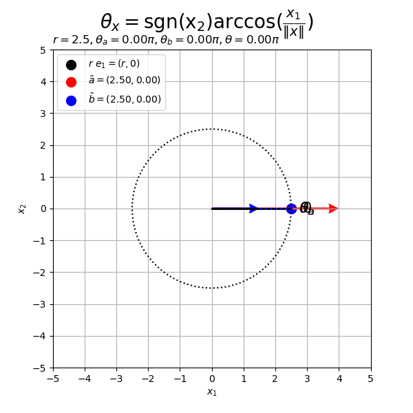
点 それぞれと点
を結ぶ半径
の円弧を描画する。
# ラベル位置の調整値を指定
d = 1.2

# 2Dベクトルとx軸を結ぶ円弧を作図
fig, ax = plt.subplots(figsize=(6, 6), facecolor='white')
ax.plot(circle_x_vals, circle_y_vals,
        color='black', linewidth=1.5, linestyle=':') # 円周
ax.plot(arc_a_x_vals, arc_a_y_vals,
        color='red', linewidth=2, linestyle='-.') # 円弧a
ax.plot(arc_b_x_vals, arc_b_y_vals,
        color='blue', linewidth=2, linestyle='--') # 円弧b
ax.scatter(r, 0,
           color='black', s=100, label='$r\ e_1 = (r, 0)$') # x軸線上の点
ax.scatter(*tilde_a,
           color='red', s=100,
           label='$\\tilde{a} = '+'({:.2f}, {:.2f})$'.format(*tilde_a)) # 点a
ax.scatter(*tilde_b,
           color='blue', s=100,
           label='$\\tilde{b} = '+'({:.2f}, {:.2f})$'.format(*tilde_b)) # 点b
ax.plot([0, r], [0, 0],
        color='black', linewidth=2) # x軸線
ax.quiver(0, 0, *a,
          color='red', units='dots', width=3, headwidth=5,
          angles='xy', scale_units='xy', scale=1) # ベクトルa
if norm_a < r:
    ax.plot([a[0], tilde_a[0]], [a[1], tilde_a[1]],
            color='red', linewidth=2, linestyle=':') # ベクトルaの延長線
ax.quiver(0, 0, *b,
          color='blue', units='dots', width=3, headwidth=5,
          angles='xy', scale_units='xy', scale=1) # ベクトルb
if norm_b < r:
    ax.plot([b[0], tilde_b[0]], [b[1], tilde_b[1]],
            color='blue', linewidth=2, linestyle=':') # ベクトルbの延長線
ax.text(d*r, 0,
        s='$0$', size=15, ha='center', va='center') # ラジアンラベルe1
ax.text(*d*tilde_a,
        s='$\\theta_a$', size=15, ha='center', va='center') # なす角aラベル
ax.text(*d*tilde_b,
        s='$\\theta_b$', size=15, ha='center', va='center') # なす角bラベル
ax.set_xticks(ticks=np.arange(x_min, x_max+1))
ax.set_yticks(ticks=np.arange(y_min, y_max+1))
ax.set_xlabel('$x_1$')
ax.set_ylabel('$x_2$')
ax.set_title('$r = {}'+str(r)+', ' +
             '\\theta_a = {:.2f} \pi'.format(theta_a/np.pi)+', ' +
             '\\theta_b = {:.2f} \pi$'.format(theta_b/np.pi), loc='left')
fig.suptitle('$\\theta = \mathrm{sgn(x_2)} \\arccos(\\frac{x_1}{\|x\|})$', fontsize=20)
ax.grid()
ax.legend()
ax.set_aspect('equal')
plt.show()

x軸線上の点 と
移動した点
をそれぞれ結んだ円弧が得られた。
なす角は劣角( から
のラジアン)なので、点
の近い方の円弧で結ぶため、(点の位置を移動せずに)角度を変換する。
# 角度の差が優角なら負の角度を優角に変換
if abs(theta_a - theta_b) > np.pi:
    theta_a = theta_a if theta_a >= 0.0 else theta_a + 2.0*np.pi
    theta_b = theta_b if theta_b >= 0.0 else theta_b + 2.0*np.pi
print(theta_a)
print(theta_b)
3.7295952571373605
2.356194490192345
角度の差の絶対値が優角( から
のラジアン)
であれば、負の角度(y座標が負の方の角度)に
を加え優角に変換して、左回りの円弧から右周りの円弧にする。
1つ前のコードで、円弧の座標を計算して、円弧を描画する(ラベルの処理は変更している)。
・作図コード(クリックで展開)
# ラベル用の文字列を作成
angle_a_label = '\\theta_a' if theta_a <= np.pi else '\\theta_a + 2 \pi'
angle_b_label = '\\theta_b' if theta_b <= np.pi else '\\theta_b + 2 \pi'

# 2Dベクトルとx軸を結ぶ円弧を作図
fig, ax = plt.subplots(figsize=(6, 6), facecolor='white')
ax.plot(circle_x_vals, circle_y_vals,
        color='black', linewidth=1.5, linestyle=':') # 円周
ax.plot(arc_a_x_vals, arc_a_y_vals,
        color='red', linewidth=2, linestyle='-.') # 円弧a
ax.plot(arc_b_x_vals, arc_b_y_vals,
        color='blue', linewidth=2, linestyle='--') # 円弧b
ax.scatter(r, 0,
           color='black', s=100, label='$r\ e_1 = (r, 0)$') # x軸線上の点
ax.scatter(*tilde_a,
           color='red', s=100,
           label='$\\tilde{a} = '+'({:.2f}, {:.2f})$'.format(*tilde_a)) # 点a
ax.scatter(*tilde_b,
           color='blue', s=100,
           label='$\\tilde{b} = '+'({:.2f}, {:.2f})$'.format(*tilde_b)) # 点b
ax.plot([0, r], [0, 0],
        color='black', linewidth=2) # x軸線
ax.quiver(0, 0, *a,
          color='red', units='dots', width=3, headwidth=5,
          angles='xy', scale_units='xy', scale=1) # ベクトルa
if norm_a < r:
    ax.plot([a[0], tilde_a[0]], [a[1], tilde_a[1]],
            color='red', linewidth=2, linestyle=':') # ベクトルaの延長線
ax.quiver(0, 0, *b,
          color='blue', units='dots', width=3, headwidth=5,
          angles='xy', scale_units='xy', scale=1) # ベクトルb
if norm_b < r:
    ax.plot([b[0], tilde_b[0]], [b[1], tilde_b[1]],
            color='blue', linewidth=2, linestyle=':') # ベクトルbの延長線
ax.text(d*r, 0,
        s='$0$', size=15, ha='center', va='center') # ラジアンラベルe1
ax.text(*d*tilde_a,
        s='$'+angle_a_label+'$', size=15, ha='center', va='center') # なす角aラベル
ax.text(*d*tilde_b,
        s='$'+angle_b_label+'$', size=15, ha='center', va='center') # なす角bラベル
ax.set_xticks(ticks=np.arange(x_min, x_max+1))
ax.set_yticks(ticks=np.arange(y_min, y_max+1))
ax.set_xlabel('$x_1$')
ax.set_ylabel('$x_2$')
ax.set_title('$r = {}'+str(r)+', ' +
             angle_a_label+'= {:.2f} \pi'.format(theta_a/np.pi)+', ' +
             angle_b_label+'= {:.2f} \pi$'.format(theta_b/np.pi), loc='left')
fig.suptitle('$\\theta = \mathrm{sgn(x_2)} \\arccos(\\frac{x_1}{\|x\|})$', fontsize=20)
ax.grid()
ax.legend()
ax.set_aspect('equal')
plt.show()

に関するそれぞれの円弧を描画した。
曲線が重ならない部分のみを描画するることで、 のなす角に対応する円弧になる。
点 を結ぶ円弧の座標を計算する。
# 円弧用のラジアンを作成
u_vals = np.linspace(start=theta_a, stop=theta_b, num=100)
print(u_vals[:5])

# 円弧の座標を計算
arc_x_vals = r * np.cos(u_vals)
arc_y_vals = r * np.sin(u_vals)
print(arc_x_vals[:5])
print(arc_y_vals[:5])
print(np.linalg.norm(np.vstack([arc_x_vals[:5], arc_y_vals[:5]]), axis=0))
[3.72959526 3.71572252 3.70184979 3.68797705 3.67410432]
[-2.08012574 -2.09916298 -2.11779624 -2.13602194 -2.15383655]
[-1.38675049 -1.35776094 -1.3285101  -1.29900358 -1.26924706]
[2.5 2.5 2.5 2.5 2.5]
から
までのラジアン
を用いて、先ほどの式で計算する。
点 を結ぶ半径
の円弧を描画する。
# 2Dベクトルを結ぶ円弧を作図
fig, ax = plt.subplots(figsize=(6, 6), facecolor='white')
ax.plot(circle_x_vals, circle_y_vals,
        color='black', linewidth=1.5, linestyle=':') # 円周
ax.plot(arc_x_vals, arc_y_vals,
        color='black', linewidth=2) # 円弧
ax.scatter(*tilde_a,
           color='red', s=100,
           label='$\\tilde{a} = '+'({:.2f}, {:.2f})$'.format(*tilde_a)) # 点a
ax.scatter(*tilde_b,
           color='blue', s=100,
           label='$\\tilde{b} = '+'({:.2f}, {:.2f})$'.format(*tilde_b)) # 点b
ax.quiver(0, 0, *a,
          color='red', units='dots', width=3, headwidth=5,
          angles='xy', scale_units='xy', scale=1) # ベクトルa
if norm_a < r:
    ax.plot([a[0], tilde_a[0]], [a[1], tilde_a[1]],
            color='red', linewidth=2, linestyle=':') # ベクトルaの延長線
ax.quiver(0, 0, *b,
          color='blue', units='dots', width=3, headwidth=5,
          angles='xy', scale_units='xy', scale=1) # ベクトルb
if norm_b < r:
    ax.plot([b[0], tilde_b[0]], [b[1], tilde_b[1]],
            color='blue', linewidth=2, linestyle=':') # ベクトルbの延長線
ax.text(*d*tilde_a,
        s='$'+angle_a_label+'$', size=15, ha='center', va='center') # なす角aラベル
ax.text(*d*tilde_b,
        s='$'+angle_b_label+'$', size=15, ha='center', va='center') # なす角bラベル
ax.set_xticks(ticks=np.arange(x_min, x_max+1))
ax.set_yticks(ticks=np.arange(y_min, y_max+1))
ax.set_xlabel('$x_1$')
ax.set_ylabel('$x_2$')
ax.set_title('$r = {}'+str(r)+', ' +
             angle_a_label+'= {:.2f} \pi'.format(theta_a/np.pi)+', ' +
             angle_b_label+'= {:.2f} \pi'.format(theta_b/np.pi)+', ' +
             '\\theta = {:.2f} \pi$'.format(abs(theta_a - theta_b)/np.pi), loc='left')
fig.suptitle('$\\theta = \\arccos(\\frac{a \cdot b}{\|a\| \|b\|})$', fontsize=20)
ax.grid()
ax.legend()
ax.set_aspect('equal')
plt.show()

サイン関数とコサイン関数は で周期する
、
ので、円周上の点の座標は
である。
以上で、円周上の2点を結ぶ円弧が得られた。
ちなみに、theta_a, theta_b の差の絶対値は、2つのベクトルのなす角と一致する。
# ベクトルa,bのなす角(ラジアン)を計算
cos_theta = np.dot(a, b) / np.linalg.norm(a) / np.linalg.norm(b)
theta = np.arccos(cos_theta)
print(theta) # 0からπの値
print(theta / np.pi) # 0から1の値
1.373400766945016
0.43716704181099886
詳しくは「なす角の描画」を参照のこと。
ベクトルの値を変化させたアニメーションを作成する。
・作図コード(クリックで展開)
# フレーム数を指定
frame_num = 60

# 変化するベクトルを作成
alpha, beta = 4.0, 1.5
rad_n = np.linspace(start=0.0, stop=2.0*np.pi, num=frame_num+1)[:frame_num]
a_n = np.array(
    [alpha * np.cos(2.0 * rad_n), alpha * np.sin(2.0 * rad_n)]
).T
b_n = np.array(
    [beta * np.cos(rad_n), beta * np.sin(rad_n)]
).T

# 半径を指定
r = 2.5

# 円周の座標を計算
t_vals = np.linspace(start=0.0, stop=2.0*np.pi, num=100)
circle_x_vals = r * np.cos(t_vals)
circle_y_vals = r * np.sin(t_vals)

# グラフサイズを設定
axis_size = np.ceil(np.max([r, abs(alpha), abs(beta)])) + 1

# グラフオブジェクトを初期化
fig, ax = plt.subplots(figsize=(6, 6), facecolor='white')
fig.suptitle('$\\theta_x = \mathrm{sgn(x_2)} \\arccos(\\frac{x_1}{\|x\|})$', fontsize=20)

# 作図処理を関数として定義
def update(i):

    # 前フレームのグラフを初期化
    plt.cla()

    # i番目のベクトルを取得
    a = a_n[i]
    b = b_n[i]

    # ノルムを調整
    tilde_a = r * a / np.linalg.norm(a)
    tilde_b = r * b / np.linalg.norm(b)

    # ベクトルa・bとx軸のなす角(ラジアン)を計算
    sgn_a   = 1.0 if a[1] >= 0.0 else -1.0
    theta_a = sgn_a * np.arccos(a[0] / np.linalg.norm(a))
    sgn_b   = 1.0 if b[1] >= 0.0 else -1.0
    theta_b = sgn_b * np.arccos(b[0] / np.linalg.norm(b))

    # 角度の差が優角なら負の角度を優角に変換
    if abs(theta_a - theta_b) > np.pi:
        theta_a = theta_a if theta_a >= 0.0 else theta_a + 2.0*np.pi
        theta_b = theta_b if theta_b >= 0.0 else theta_b + 2.0*np.pi

    # なす角a・bの円弧の座標を計算
    u_a_vals = np.linspace(start=0.0, stop=theta_a, num=100)
    arc_a_x_vals = r * np.cos(u_a_vals)
    arc_a_y_vals = r * np.sin(u_a_vals)
    u_b_vals = np.linspace(start=0.0, stop=theta_b, num=100)
    arc_b_x_vals = r * np.cos(u_b_vals)
    arc_b_y_vals = r * np.sin(u_b_vals)

    # 円弧の座標を計算
    u_vals = np.linspace(start=theta_a, stop=theta_b, num=100)
    arc_x_vals = r * np.cos(u_vals)
    arc_y_vals = r * np.sin(u_vals)

    # ラベル用の文字列を作成
    angle_a_label = '\\theta_a' if theta_a <= np.pi else '\\theta_a + 2 \pi'
    angle_b_label = '\\theta_b' if theta_b <= np.pi else '\\theta_b + 2 \pi'

    # 2Dベクトルを結ぶ円弧を作図
    d = 1.2
    e = 0.05
    ax.plot(circle_x_vals, circle_y_vals,
            color='black', linewidth=1.5, linestyle=':') # 円周
    ax.plot(arc_a_x_vals*(1.0+e), arc_a_y_vals*(1.0+e),
            color='red', linewidth=3) # 円弧a
    ax.plot(arc_b_x_vals*(1.0-e), arc_b_y_vals*(1.0-e),
            color='blue', linewidth=3) # 円弧b
    ax.plot(arc_x_vals, arc_y_vals,
            color='black', linewidth=3) # 円弧
    ax.scatter(r, 0,
               color='black', s=100, label='$r\ e_1 = (r, 0)$') # x軸線上の点
    ax.scatter(*tilde_a,
               color='red', s=100,
               label='$\\tilde{a} = '+'({: .2f}, {: .2f})$'.format(*tilde_a)) # 点a
    ax.scatter(*tilde_b,
               color='blue', s=100,
               label='$\\tilde{b} = '+'({: .2f}, {: .2f})$'.format(*tilde_b)) # 点b
    ax.plot([0, r], [0, 0],
            color='black', linewidth=2) # x軸線
    ax.quiver(0, 0, *a,
              color='red', units='dots', width=3, headwidth=5,
              angles='xy', scale_units='xy', scale=1) # ベクトルa
    if np.linalg.norm(a) < r:
        ax.plot([a[0], tilde_a[0]], [a[1], tilde_a[1]],
                color='red', linewidth=2, linestyle=':') # ベクトルaの延長線
    ax.quiver(0, 0, *b,
              color='blue', units='dots', width=3, headwidth=5,
              angles='xy', scale_units='xy', scale=1) # ベクトルb
    if np.linalg.norm(b) < r:
        ax.plot([b[0], tilde_b[0]], [b[1], tilde_b[1]],
                color='blue', linewidth=2, linestyle=':') # ベクトルbの延長線
    ax.text(d*r, 0,
            s='$0$', size=15, ha='center', va='center') # ラジアンラベルe1
    ax.text(*d*tilde_a,
            s='$'+angle_a_label+'$', size=15, ha='center', va='center') # なす角aラベル
    ax.text(*d*tilde_b,
            s='$'+angle_b_label+'$', size=15, ha='center', va='center') # なす角bラベル
    ax.set_xticks(ticks=np.arange(-axis_size, axis_size+1))
    ax.set_yticks(ticks=np.arange(-axis_size, axis_size+1))
    ax.set_xlabel('$x_1$')
    ax.set_ylabel('$x_2$')
    ax.set_title('$r = {}'+str(r)+', ' +
                 angle_a_label+'= {: .2f} \pi'.format(theta_a/np.pi)+', ' +
                 angle_b_label+'= {: .2f} \pi'.format(theta_b/np.pi)+', ' +
                 '\\theta = {: .2f} \pi$'.format(abs(theta_a - theta_b)/np.pi), loc='left')
    ax.grid()
    ax.legend(loc='upper left')
    ax.set_aspect('equal')

# gif画像を作成
ani = FuncAnimation(fig=fig, func=update, frames=frame_num, interval=100)

# gif画像を保存
ani.save(filename='2d_arc_ab.gif')
ベクトル の位置関係によって円弧を描画する向きが変わるのが分かる(伝わってほしい)。
この記事では、2次元空間における2つの線分を結ぶ曲線を扱った。次の記事では、3次元空間における2つの線分を結ぶ曲線を扱う。
おわりに
なんでかとっても難産でした。同時並行して書いてた記事がいくつかあったのでそっちを先に書き終えようと後回しにしたら、そのまま放置して3か月が経ってました。書きたいことをいくつか分割して、別記事や別章にしたらなんとか書けました。
これで頭の隅にずっとあったモヤモヤが1つ晴れました。
ところで未だに角マークや角度マークと呼んでるアレの正式名称が分かりません。マークじゃなくてシンボルかもしれない。本当は塗り潰した方がいいのかもしれないとも思い始めました。誰か教えてください。
それともっと良い実装方法があれば教えてください。
2023年8月4日は、エビ中こと私立恵比寿中学の結成14周年の日です。
私はハマって1年経ったか足らずな新参ですが、ここまで続けてくれていたから出会えました!ありがとうございます。これからもよろしくお願いします。
【次の内容】