はじめに

　R言語のgganimateパッケージを使ってグラフを動かそうシリーズです。
　この記事では、全ての方向に移動する2次元のランダムウォークのアニメーションを作成します。

【前の内容】

【他の内容】

【目次】

はじめに
2次元ランダムウォークの作図：全方向移動
おわりに

2次元ランダムウォークの作図：全方向移動

　平面上の全ての方向(360°)に移動するランダムウォーク(random walk)のアニメーションを作成します。
　gganimate パッケージの関数 transition_reveal() については、「transition_reveal関数【gganimate】 - からっぽのしょこ」を参照してください。

　利用するパッケージを読み込みます。

# 利用パッケージ
library(gganimate)
library(tidyverse)

　この記事では、基本的に パッケージ名::関数名() の記法を使うので、パッケージの読み込みは不要です。ただし、作図コードについてはパッケージ名を省略するので、ggplot2 を読み込む必要があります。
　また、ネイティブパイプ演算子 |> を使います。magrittr パッケージのパイプ演算子 %>% に置き換えられますが、その場合は magrittr を読み込む必要があります。

全方向移動の確認

　まずは、平面上を移動する処理を確認します。
　円周の座標計算やラジアンについては「【R】円周の作図 - からっぽのしょこ」を参照してください。

・作図コード(クリックで展開)

　単位円の円周上の点の座標を計算します。

# フレーム数を指定
frame_num <- 101

# 単位円周上の点を作成
point_df <- tibble::tibble(
  frame_i = 1:frame_num, # フレーム番号(時計回りならframe_num:1)
  t = seq(from = 0, to = 2*pi, length.out = frame_num+1)[1:frame_num], # 1周分のラジアン
  x = cos(t), 
  y = sin(t), 
  label = paste0(
    "list(", 
    "t == ", round(t/pi, digits = 2), "*pi, ", 
    "(list(x, y)) == (list(", round(x, digits = 2), ", ", round(y, digits = 2), "))", 
    ")"
  )
)
point_df

# A tibble: 101 × 5
   frame_i      t     x      y label                                            
     <int>  <dbl> <dbl>  <dbl> <chr>                                            
 1       1 0      1     0      list(t == 0*pi, (list(x, y)) == (list(1, 0)))    
 2       2 0.0622 0.998 0.0622 list(t == 0.02*pi, (list(x, y)) == (list(1, 0.06…
 3       3 0.124  0.992 0.124  list(t == 0.04*pi, (list(x, y)) == (list(0.99, 0…
 4       4 0.187  0.983 0.186  list(t == 0.06*pi, (list(x, y)) == (list(0.98, 0…
 5       5 0.249  0.969 0.246  list(t == 0.08*pi, (list(x, y)) == (list(0.97, 0…
 6       6 0.311  0.952 0.306  list(t == 0.1*pi, (list(x, y)) == (list(0.95, 0.…
 7       7 0.373  0.931 0.365  list(t == 0.12*pi, (list(x, y)) == (list(0.93, 0…
 8       8 0.435  0.907 0.422  list(t == 0.14*pi, (list(x, y)) == (list(0.91, 0…
 9       9 0.498  0.879 0.477  list(t == 0.16*pi, (list(x, y)) == (list(0.88, 0…
10      10 0.560  0.847 0.531  list(t == 0.18*pi, (list(x, y)) == (list(0.85, 0…
# ℹ 91 more rows

　フレーム数 frame_num を指定して、frame_num 個の点の座標を作成します。
　 $0$ から $2 \pi$ の値 $t$ を作成して、x軸の値を $x = \cos t$ 、y軸の値を $y = \sin r$ で計算します。 $\pi$ は円周率で、pi で扱えます。

　ノルム目盛線(円周)の描画用のデータフレームを作成します。

# グラフサイズを設定
axis_size <- 1

# 目盛間隔を設定
tick_major_val <- 0.5
tick_minor_val <- 0.5 * tick_major_val

# ノルム目盛線の座標を作成
circle_df <- tidyr::expand_grid(
  r = seq(from = tick_minor_val, to = axis_size, by = tick_minor_val), # 半径
  t = seq(from = 0, to = 2*pi, length.out = 361), # 1周期分のラジアン
) |> # ノルムごとにラジアンを複製
  dplyr::mutate(
    x = r * cos(t), 
    y = r * sin(t), 
    grid  = dplyr::if_else(
      r%%tick_major_val == 0, true = "major", false = "minor"
    ) # 目盛カテゴリ
  ) # 円周の座標を計算
circle_df

# A tibble: 1,444 × 5
       r      t     x       y grid 
   <dbl>  <dbl> <dbl>   <dbl> <chr>
 1  0.25 0      0.25  0       minor
 2  0.25 0.0175 0.250 0.00436 minor
 3  0.25 0.0349 0.250 0.00872 minor
 4  0.25 0.0524 0.250 0.0131  minor
 5  0.25 0.0698 0.249 0.0174  minor
 6  0.25 0.0873 0.249 0.0218  minor
 7  0.25 0.105  0.249 0.0261  minor
 8  0.25 0.122  0.248 0.0305  minor
 9  0.25 0.140  0.248 0.0348  minor
10  0.25 0.157  0.247 0.0391  minor
# ℹ 1,434 more rows

　グラフサイズ axis_size と主目盛の間隔 tick_major_val を指定して、目盛線の間隔に応じた半径の円周の座標を作成します。

　角度目盛線(中心を通る斜線)の描画用のデータフレームを作成します。

# 半円(範囲π)における目盛数を指定
tick_num <- 6

# 角度目盛線の座標を作成
diag_df <- tibble::tibble(
  i = seq(from = 0, to = tick_num-0.5, by = 0.5), # 目盛番号
  t = i/tick_num * pi, # 半周期分のラジアン
  a = tan(t), # 目盛線の傾き
  grid = dplyr::if_else(
    i%%1 == 0, true = "major", false = "minor"
  ) # 目盛カテゴリ
)
diag_df

# A tibble: 12 × 4
       i     t         a grid 
   <dbl> <dbl>     <dbl> <chr>
 1   0   0      0        major
 2   0.5 0.262  2.68e- 1 minor
 3   1   0.524  5.77e- 1 major
 4   1.5 0.785  1   e+ 0 minor
 5   2   1.05   1.73e+ 0 major
 6   2.5 1.31   3.73e+ 0 minor
 7   3   1.57   1.63e+16 major
 8   3.5 1.83  -3.73e+ 0 minor
 9   4   2.09  -1.73e+ 0 major
10   4.5 2.36  -1   e+ 0 minor
11   5   2.62  -5.77e- 1 major
12   5.5 2.88  -2.68e- 1 minor

　半円における目盛数 tick_num を指定して、目盛線の角度(円周上の点に対応する偏角) t を用いて目盛線の傾き a を作成します。

　作成した点を描画します。

# 単位円周上の点を作図
anim <- ggplot() + 
  geom_path(data = circle_df, 
            mapping = aes(x = x, y = y, linewidth = grid, group = r), 
            color = "white", show.legend = FALSE) + # ノルム目盛線
  geom_abline(data = diag_df, 
              mapping = aes(slope = a, intercept = 0, linewidth = grid), 
              color = "white", show.legend = FALSE) + # 角度目盛線
  geom_segment(data = point_df, 
               mapping = aes(x = 0, y = 0, xend = x, yend = y), 
               linewidth = 1) + # 動径
  geom_point(data = point_df, 
             mapping = aes(x = x, y = y), 
             size = 4) + # 円周上の点
  geom_text(data = point_df, 
            mapping = aes(x = -Inf, y = Inf, label = label), 
            parse = TRUE, hjust = 0, vjust = -0.5) + # 座標ラベル(subtitleの代用)
  gganimate::transition_manual(frames = frame_i) + # フレーム切替
  scale_linewidth_manual(breaks = c("major", "minor"), 
                         values = c(0.5, 0.25)) + # 主・補助目盛線用
  coord_fixed(ratio = 1, clip = "off") + # アスペクト比
  labs(title = "unit circle", 
       subtitle = "", # ラベル用の空行
       x = expression(x == cos~t), 
       y = expression(y == sin~t))

# gif画像を作成
gganimate::animate(
  plot = anim, nframes = frame_num, fps = 10, 
  width = 5, height = 5, units = "in", res = 250
)

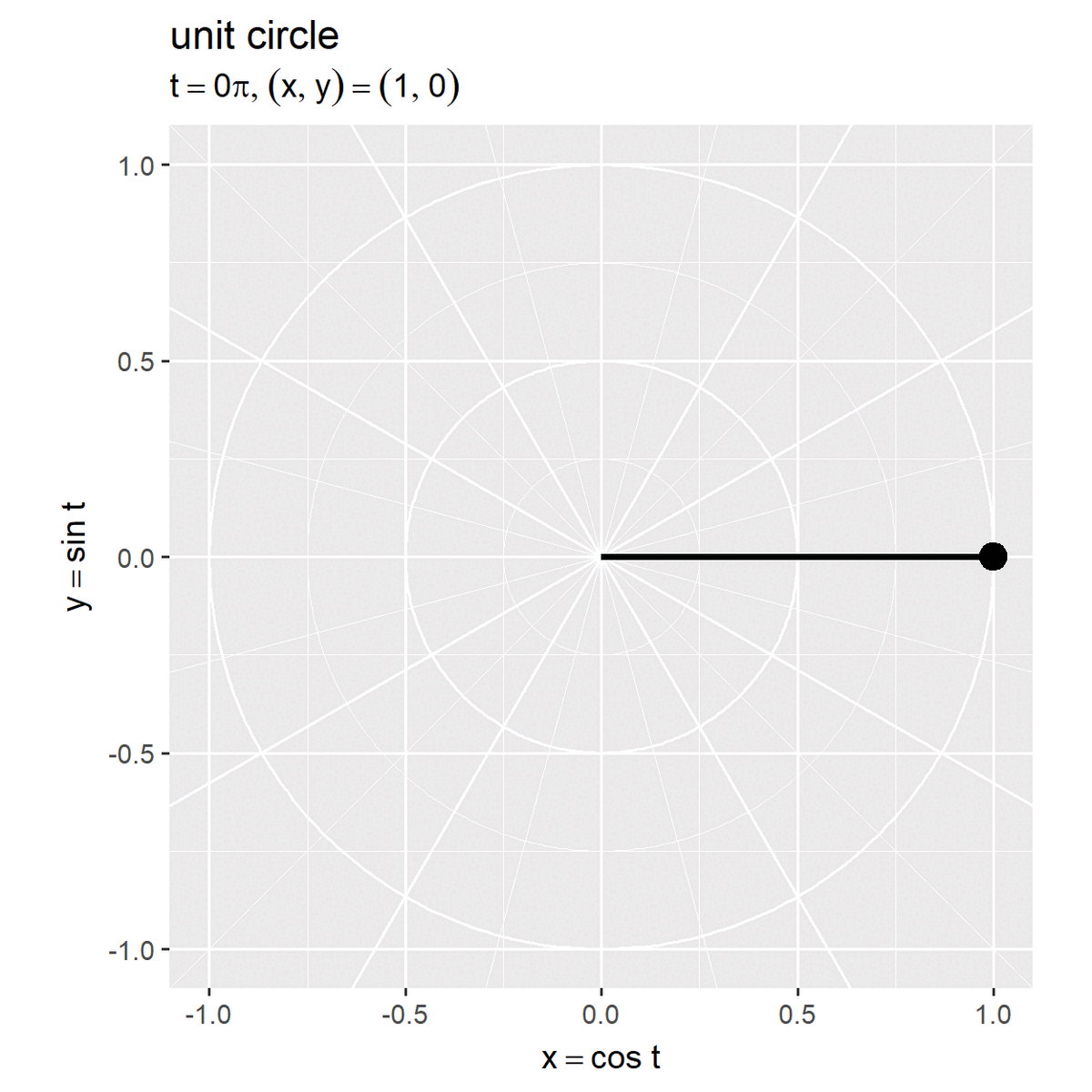
　ラジアン(弧度法の角度) $0 \leq t \lt 2 \pi$ を用いて $(x, y) = (\cos t, \sin t)$ が単位円(半径が1)の円周上の点になります。 $\pi$ は円周率。
　つまり、 $0$ から $2 \pi$ の乱数を生成して座標を計算すると、現在の位置(円の中心)からランダムな方向に距離(ノルム)1の移動を表せます。

1サンプル

　次は、1つのサンプルを描画します。

　試行回数を指定して、移動量の計算用の値をランダムに生成します。

# 試行回数を指定
max_iter <- 100

# 移動量用の乱数を生成
random_vec <- 2*pi * runif(n = max_iter, min = 0, max = 1) # 0から2π
head(random_vec)

[1] 3.517173 1.058621 4.948280 4.560863 1.162678 4.511959

　 $0$ から $2 \pi$ の一様乱数を runif()で生成します。 $\pi$ は円周率で、pi で扱えます。最小値の引数 min に 0、最大値の引数 max に 1 を指定して、2*pi を掛けます。または、max 引数に 2*pi を指定します。
　この例では原理的な処理が分かりやすいように、0 から 1 の乱数に 2*pi を掛けることで $0$ から $2 \pi$ の乱数を作成しています。(本当は0以上1未満の乱数を生成しないといけませんが、やり方が分かりませんでした。)

　移動量に応じた座標を計算します。

# 試行ごとに集計
trace_df <- tibble::tibble(
  iter = 0:max_iter, # 試行番号
  x    = c(0, cos(random_vec)), # 移動量のx座標
  y    = c(0, sin(random_vec))  # 移動量のy座標
) |> 
  dplyr::mutate(
    x = cumsum(x), 
    y = cumsum(y)
  ) # 総移動量を計算
trace_df

# A tibble: 101 × 3
    iter       x      y
   <int>   <dbl>  <dbl>
 1     0  0       0    
 2     1 -0.930  -0.367
 3     2 -0.440   0.505
 4     3 -0.207  -0.467
 5     4 -0.357  -1.46 
 6     5  0.0394 -0.538
 7     6 -0.160  -1.52 
 8     7 -1.05   -1.96 
 9     8 -0.983  -2.96 
10     9 -1.55   -2.14 
# ℹ 91 more rows

　乱数を用いてx座標を cos()、y座標を sin() で計算します。
　初期値(スタート地点・0回目の結果)を 0 として追加して、各試行までの和(累積和)を cumsum() で計算します。

　点の推移のアニメーションを作成します。

# 最大移動量を取得
max_val <- c(trace_df[["x"]], trace_df[["y"]]) |> 
  abs() |> 
  max()

# 目盛間隔を設定
tick_major_val <- 5
tick_minor_val <- 0.5 * tick_major_val

# グラフサイズを設定:(目盛間隔で切り上げ)
axis_size <- ceiling(max_val / tick_minor_val) * tick_minor_val

# ノルム目盛線の座標を作成
circle_df <- tidyr::expand_grid(
  r = seq(from = tick_minor_val, to = axis_size, by = tick_minor_val), # 半径
  t = seq(from = 0, to = 2*pi, length.out = 361), # 1周期分のラジアン
) |> # ノルムごとにラジアンを複製
  dplyr::mutate(
    x = r * cos(t), 
    y = r * sin(t), 
    grid  = dplyr::if_else(
      r%%tick_major_val == 0, true = "major", false = "minor"
    ) # 目盛カテゴリ
  ) # 円周の座標を計算

# 2次元ランダムウォークのアニメーションを作図
anim <- ggplot() + 
  geom_path(data = circle_df, 
            mapping = aes(x = x, y = y, linewidth = grid, group = r), 
            color = "white", show.legend = FALSE) + # ノルム目盛線
  geom_abline(data = diag_df, 
              mapping = aes(slope = a, intercept = 0, linewidth = grid), 
              color = "white", show.legend = FALSE) + # 角度目盛線
  geom_path(data = trace_df, 
            mapping = aes(x = x, y = y), 
            size = 1) + # 軌跡
  geom_point(data = trace_df, 
             mapping = aes(x = x, y = y), 
             size = 4) + # 現在地点
  geom_hline(yintercept = 0, color = "red", linetype = "dashed") + # 初期値
  geom_vline(xintercept = 0, color = "red", linetype = "dashed") + # 初期値
  gganimate::transition_reveal(along = iter) + # フレーム切替
  scale_linewidth_manual(breaks = c("major", "minor"), 
                         values = c(0.5, 0.25)) + # 主・補助目盛線用
  coord_fixed(ratio = 1, 
              xlim = c(-axis_size, axis_size), 
              ylim = c(-axis_size, axis_size)) + # アスペクト比
  labs(title = "Random Walk", 
       subtitle = "iteration: {frame_along}", 
       x = "x", y = "y")

# gif動画を作成
gganimate::animate(
  plot = anim, nframes = max_iter+1, fps = 10, 
  width = 8, height = 8, units = "in", res = 250
)

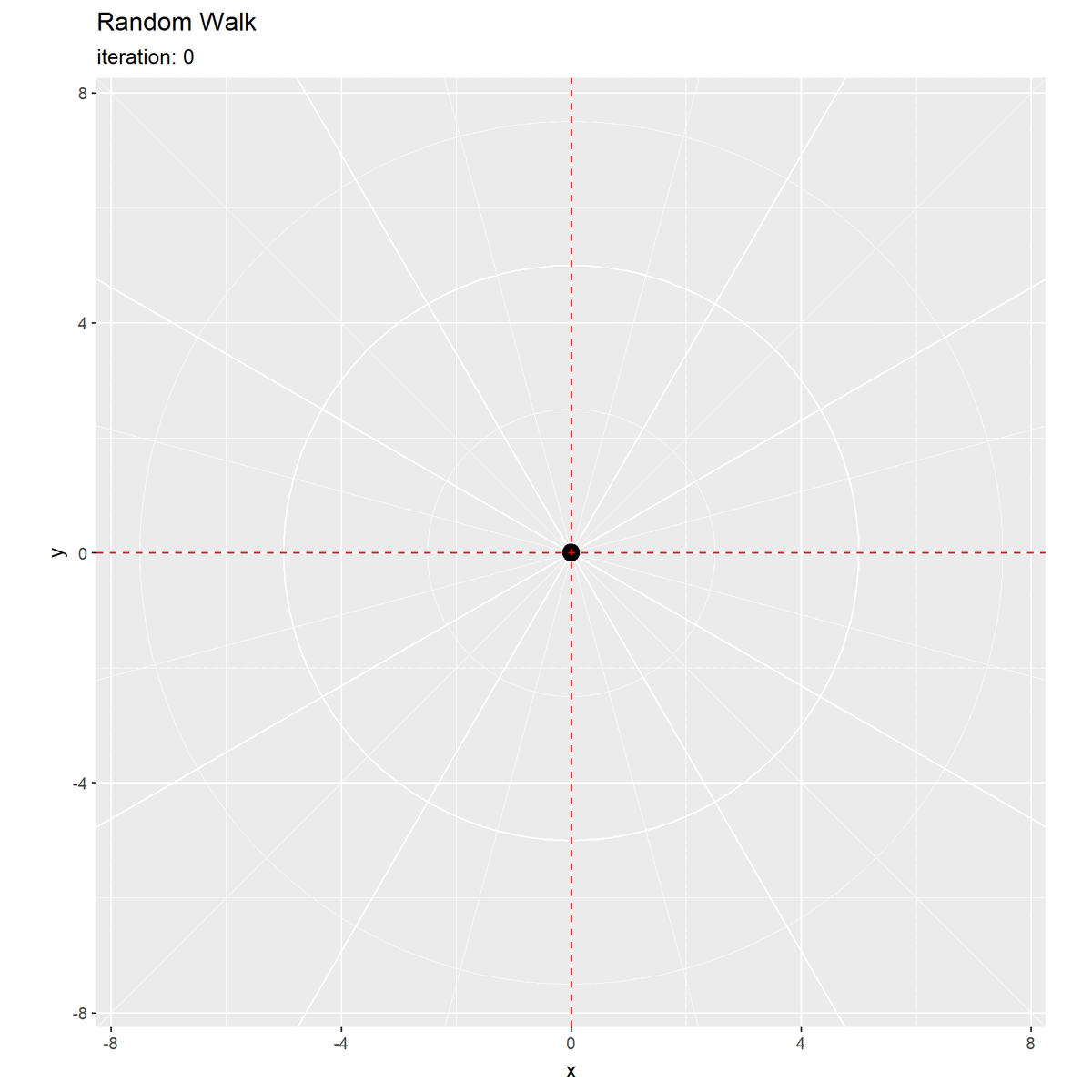
　初期値(期待値)を破線で示します。

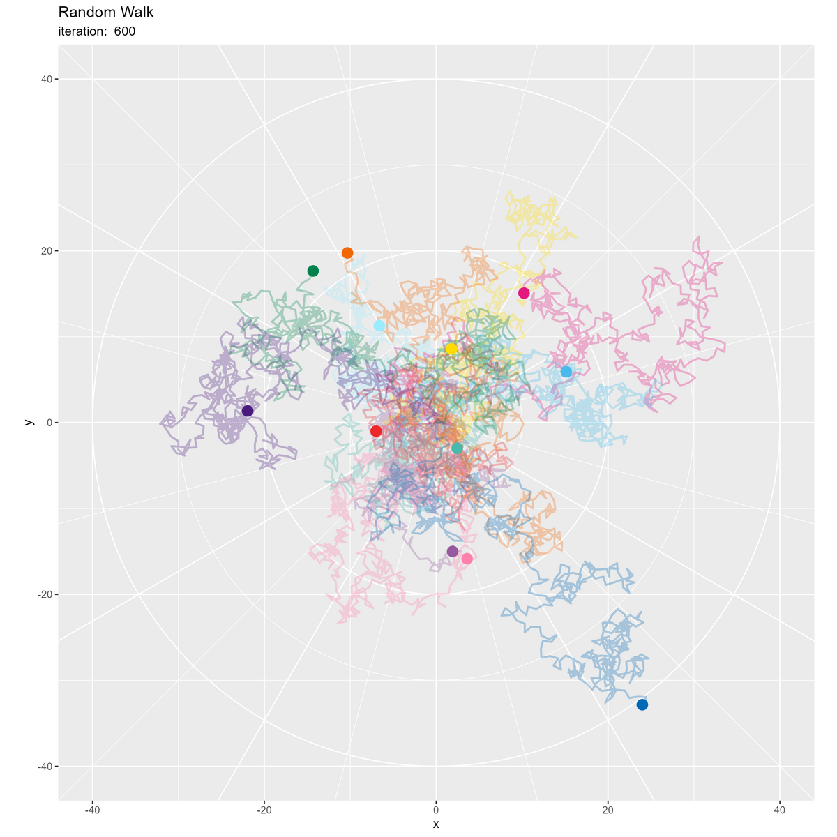
複数サンプル

　続いて、複数のサンプルを並べて描画します。
　作図コードについては「GitHub - anemptyarchive/gganimate/.../RandomWalk.R」を参照してください。

・最終結果

・推移のアニメーション

　等確率で移動する場合、初期値が期待値になりますが分散を持ち(散らばり)ます。

　この記事では、平面上の全ての方向に移動する2次元のランダムウォークを扱いました。

おわりに

　試作段階では酷いコードだったんですが、清書してると思いの外きれいに処理できて良かったです。

2024.02.14：加筆修正しました。

　Twitterがアレなんでいくつか他にアカウントを作りまして、自己紹介がてらにこの図を投稿しようと思い作り直しました。
　(既に使われていて泣くなく1文字足した1つを除いて)はてなIDと同じIDでやってる(投稿してるとは言ってない)のでよければフォローしてください。運用方針が定まればプロフィールページに一覧でリンクします。今のところメインはTwitterです。

　元記事を書いた時点では、360°移動の処理に悩んだ記憶があります。その後、円関数(三角関数)について勉強することになって理解できました。今回の修正では、円関数関連の記事での内容や処理を流用することで分かりやすくなったと思います。別で学んだ知識が繋がると嬉しいです。

【次の記事】

3次元版を(Pythonで)作成中です

からっぽのしょこ

読んだら書く！書いたら読む！同じ事は二度調べ(たく)ない

【R】2次元ランダムウォークの作図：全方向移動【gganimate】