はじめに

　円関数(三角関数)の定義や性質、公式などを可視化して理解しようシリーズです。

　この記事では、一般角の符号の反転と円関数の関係のグラフを作成します。

【前の内容】

www.anarchive-beta.com

【他の内容】

www.anarchive-beta.com

【この記事の内容】

はじめに
-θ(負角)の可視化
- 定義式の確認
- 単位円と関数の関係
  - グラフの作成
  - アニメーションの作成
おわりに

-θ(負角)の可視化

　負の角度(負角・negative angle)について、単位円における定義をグラフで確認します。また、変数(偏角)の符号を反転したときの円関数(circular functions)・三角関数(trigonometric functions)との関係を確認します。
　度数法と弧度法(角度とラジアン)の関係や単位円における偏角については「【R】円周の作図 - からっぽのしょこ」を参照してください。

　利用するパッケージを読み込みます。

# 利用パッケージ
library(tidyverse)

　この記事では、基本的に パッケージ名::関数名() の記法を使うので、パッケージの読み込みは不要です。ただし、作図コードについてはパッケージ名を省略するので、ggplot2 を読み込む必要があります。
　また、ネイティブパイプ演算子 |> を使います。magrittr パッケージのパイプ演算子 %>% に置き換えられますが、その場合は magrittr を読み込む必要があります。

定義式の確認

　まずは、負角の定義と円関数との関係を数式で確認します。
　各関数についてはそれぞれの記事を参照してください。

　負の値の角度 $\theta \lt 0$ を負角と呼びます。
　ここでは、(負の値を含む)ある角度 $\theta$ に関して、符号を反転した角度 $\tau$ について考えます。

$\displaystyle \tau = - \theta$

　変数 $\theta, \tau$ はラジアン(弧度法の角度)で、鋭角 $0 \lt \theta \lt \frac{\pi}{2}$ (度数法の角度だと $0^{\circ} \lt \theta^{\circ} \lt 90^{\circ}$ )の範囲外も扱います。 $\pi$ は円周率です。

　sin関数とcos関数に関して、2つの角度は、次の関係になります。

$\displaystyle \begin{aligned} \sin (- \theta) &= - \sin \theta \\ \cos (- \theta) &= \cos \theta \end{aligned}$

　sin関数は符号が反転した値と一致し、cos関数は値が変わりません。
　この関係を用いると、sin関数またはcos関数を用いて定義される関数

$\displaystyle \begin{aligned} \tan x &= \frac{\sin x}{\cos x} \\ \cot x &= \frac{\cos x}{\sin x} \\ \sec x &= \frac{1}{\cos x} \\ \csc x &= \frac{1}{\sin x} \end{aligned}$

は、次の関係になります。

$\displaystyle \begin{aligned} \tan (- \theta) &= \frac{\sin (- \theta)}{\cos (- \theta)} = \frac{- \sin \theta}{\cos \theta} = - \tan \theta \\ \cot (- \theta) &= \frac{\cos (- \theta)}{\sin (- \theta)} = \frac{\cos \theta}{- \sin \theta} = - \cot \theta \\ \sec (- \theta) &= \frac{1}{\cos (- \theta)} = \frac{1}{\cos \theta} = \sec \theta \\ \csc (- \theta) &= \frac{1}{\sin (- \theta)} = \frac{1}{- \sin \theta} = - \csc \theta \end{aligned}$

　定義にsin関数を含む関数は符号が反転します。

単位円と関数の関係

　次は、単位円における偏角(単位円周上の点)と円関数(sin・cos)の関係を可視化します。

グラフの作成

　変数を固定して、単位円における偏角のグラフを作成します。

・作図コード(クリックで展開)

　基準となる角度を指定し対象の角度を計算して、円周上の点の描画用のデータフレームを作成します。

# 点用のラジアンを指定
theta <- 2/6 * pi

# 符号を反転
tau <- -theta

# 円周上の点の座標を作成
point_df <- tibble::tibble(
  t = c(theta, tau), 
  x = cos(t), 
  y = sin(t), 
  type = c("main", "target") # 角度カテゴリ
)
point_df

# A tibble: 2 × 4
      t     x      y type  
  <dbl> <dbl>  <dbl> <chr> 
1  1.05   0.5  0.866 main  
2 -1.05   0.5 -0.866 target

　変数(ラジアン) $\theta$ を指定して、符号を反転 $\tau = -\theta$ します。
　2つの偏角 $t = \theta, \tau$ について、単位円の円周上の点の座標 $(x, y) = (\cos t, \sin t)$ を計算します。

　偏角を示す線分の描画用のデータフレームを作成します。

# 半径線の終点の座標を作成
radius_df <- dplyr::bind_rows(
  # 始線
  tibble::tibble(
    x = 1, 
    y = 0, 
    type = "main" # 角度カテゴリ
  ), 
  # 動径線
  point_df |> 
    dplyr::select(x, y, type)
)
radius_df

# A tibble: 3 × 3
      x      y type  
  <dbl>  <dbl> <chr> 
1   1    0     main  
2   0.5  0.866 main  
3   0.5 -0.866 target

　原点と点 $(1, 0)$ を結ぶ線分(始線)、原点と点 $(\cos t, \sin t)$ を結ぶ線分(動径線)用に、円周上の点の座標を格納します。原点 $(0, 0)$ の座標は、作図時に引数に直接指定します。

　角マークの描画用のデータフレームを作成します。

# 角マークの座標を作成
ds <- 0.005
angle_mark_df <- tibble::tibble(
  t    = c(theta, tau), 
  type = c("main", "target"), # 角度カテゴリ
  d    = c(0.15, 0.25) # マークサイズを指定
) |> 
  dplyr::reframe(
    u = seq(from = 0, to = t, length.out = 600), .by = dplyr::everything()
  ) |> # 円弧用のラジアンを作成
  dplyr::mutate(
    x = (d + ds*u) * cos(u), 
    y = (d + ds*u) * sin(u)
  )
angle_mark_df

# A tibble: 1,200 × 6
       t type      d       u     x        y
   <dbl> <chr> <dbl>   <dbl> <dbl>    <dbl>
 1  1.05 main   0.15 0       0.15  0       
 2  1.05 main   0.15 0.00175 0.150 0.000262
 3  1.05 main   0.15 0.00350 0.150 0.000525
 4  1.05 main   0.15 0.00524 0.150 0.000787
 5  1.05 main   0.15 0.00699 0.150 0.00105 
 6  1.05 main   0.15 0.00874 0.150 0.00131 
 7  1.05 main   0.15 0.0105  0.150 0.00157 
 8  1.05 main   0.15 0.0122  0.150 0.00184 
 9  1.05 main   0.15 0.0140  0.150 0.00210 
10  1.05 main   0.15 0.0157  0.150 0.00236 
# ℹ 1,190 more rows

　2つの偏角 $t$ を示す角マークとして、 $0 \leq u \leq t$ のラジアンを作成して、係数が $d$ の螺旋の座標 $(x, y) = (d u \cos u, d u \sin u)$ を計算します。この例では、ノルムの基準値 d と間隔用の係数 ds でサイズを調整します。ds を 0 にすると、半径が $d$ の円弧の座標 $(x, y) = (d \cos u, d \sin u)$ になります。

　角ラベルの描画用のデータフレームを作成します。

# 角ラベルの座標を作成
angle_label_df <- tibble::tibble(
  d = c(0.1, 0.3), # ラベル位置を指定
  u = 0.5 * c(theta, tau), 
  x = d * cos(u), 
  y = d * sin(u), 
  angle_label = c("theta", "tau")
)
angle_label_df

# A tibble: 2 × 5
      d      u      x     y angle_label
  <dbl>  <dbl>  <dbl> <dbl> <chr>      
1   0.1  0.524 0.0866  0.05 theta      
2   0.3 -0.524 0.260  -0.15 tau

　角マークの中点に角ラベルを配置することにします。 $u = \frac{t}{2}$ のラジアンを作成して、円弧上の点の座標を計算します。原点からのノルム d で表示位置を調整します。

　関数を示す線分の描画用のデータフレームを作成します。

# 関数の描画順を指定
fnc_level_vec <- c("sin", "cos")

# 関数線分の座標を作成
fnc_seg_df <- tibble::tibble(
  fnc = c(
    "sin", "cos", "sin", "cos", 
    "sin", "cos"
  ) |> 
    factor(levels = fnc_level_vec), # 関数カテゴリ
  type = c(
    "main", "main", "main", "main", 
    "target", "target"
  ), # 角度カテゴリ
  x_from = c(
    cos(theta), 0, 0, 0, 
    cos(tau), 0
  ), 
  y_from = c(
    0, 0, 0, sin(theta), 
    0, 0
  ), 
  x_to = c(
    cos(theta), cos(theta), 0, cos(theta), 
    cos(tau), cos(tau)
  ), 
  y_to = c(
    sin(theta), 0, sin(theta), sin(theta), 
    sin(tau), 0
  )
)
fnc_seg_df

# A tibble: 6 × 6
  fnc   type   x_from y_from  x_to   y_to
  <fct> <chr>   <dbl>  <dbl> <dbl>  <dbl>
1 sin   main      0.5  0       0.5  0.866
2 cos   main      0    0       0.5  0    
3 sin   main      0    0       0    0.866
4 cos   main      0    0.866   0.5  0.866
5 sin   target    0.5  0       0.5 -0.866
6 cos   target    0    0       0.5  0

　各線分(の長さ)に対応する関数カテゴリを fnc 列として線の描き分けなどに使います。線分の描画順(重なり順や色付け順)を因子レベルで設定します。
　各線分の始点の座標を x_from, y_from 列、終点の座標を x_to, y_to 列として、完成図を見ながら頑張って格納します。

　関数ラベルの描画用のデータフレームを作成します。

# 関数ラベルの座標を作成
fnc_label_df <- tibble::tibble(
  fnc = c(
    "sin", "cos", 
    "sin", "cos"
  ) |> 
    factor(levels = fnc_level_vec), # 関数カテゴリ
  x = c(
    cos(theta), 0.5*cos(theta), 
    cos(tau), 0.5*cos(tau)
  ), 
  y = c(
    0.5*sin(theta), 0, 
    0.5*sin(tau), 0
  ), 
  fnc_label = c(
    "sin~theta", "cos~theta", 
    "sin~tau", "cos~tau"
  ), 
  a = c(
    90, 0, 
    90, 0
  ), 
  h = 0.5, 
  v = c(
    -0.5, -0.5, 
    1.5, 1.5
  )
)
fnc_label_df

# A tibble: 4 × 7
  fnc       x      y fnc_label     a     h     v
  <fct> <dbl>  <dbl> <chr>     <dbl> <dbl> <dbl>
1 sin    0.5   0.433 sin~theta    90   0.5  -0.5
2 cos    0.25  0     cos~theta     0   0.5  -0.5
3 sin    0.5  -0.433 sin~tau      90   0.5   1.5
4 cos    0.25  0     cos~tau       0   0.5   1.5

　偏角と関数の組み合わせごとに1つの線分の中点に関数名を表示することにします。
　ラベルの表示角度を a 列、表示角度に応じた左右の表示位置を h 列、上下の表示位置を v 列として指定します。

　各種ラベルの表示用の文字列を作成します。

# ラベル用の文字列を作成
def_label <- paste0(
  "list(", 
  "tau == - theta, ", 
  "sin(-theta) == -sin~theta, ", 
  "cos(-theta) == cos~theta", 
  ")"
)
angle_label_vec <- paste(
  c("theta", "tau"), 
  c(theta/pi, tau/pi) |> 
    round(digits = 2), 
  sep = " == "
) |> 
  paste("* pi")
fnc_label_vec <- paste(
  c("sin~theta", "cos~theta"), 
  c(sin(theta), cos(theta)) |> 
    round(digits = 2), 
  sep = " == "
)
def_label; angle_label_vec

[1] "list(tau == - theta, sin(-theta) == -sin~theta, cos(-theta) == cos~theta)"
[1] "theta == 0.33 * pi" "tau == -0.33 * pi"

　サブタイトル用の変数ラベル、凡例用の関数ラベルを作成します。
　ラベルとして数式(ギリシャ文字や記号)を表示する場合は、expression() の記法を用います。その際に、オブジェクト(プログラム上の変数)を使う場合は、文字列として作成しておき parse() の text 引数に渡します。

　単位円と角度(ラジアン)目盛の描画用のデータフレームを作成します。

# 円周の座標を作成
circle_df <- tibble::tibble(
  t = seq(from = 0, to = 2*pi, length.out = 361), # 1周期分のラジアン
  r = 1, # 半径
  x = r * cos(t), 
  y = r * sin(t)
)

# 半円(範囲π)における目盛数(分母の値)を指定
tick_num <- 6

# 角度目盛の座標を作成:(補助目盛有り)
d <- 1.1
rad_tick_df <- tibble::tibble(
  # 座標用
  i     = seq(from = 0, to = 2*tick_num-0.5, by = 0.5), # 目盛番号(分子の値)
  t_deg = i/tick_num * 180, # 度数法の角度
  t_rad = i/tick_num * pi,  # 弧度法の角度(ラジアン)
  r     = 1, # 半径
  x     = r * cos(t_rad), 
  y     = r * sin(t_rad), 
  major_flag = i%%1 == 0, # 主・補助フラグ
  grid       = dplyr::if_else(major_flag, true = "major", false = "minor"), # 目盛カテゴリ
  # ラベル用
  rad_label  = dplyr::if_else(
    major_flag, true = paste0("frac(", i, ", ", tick_num, ") ~ pi"), false = ""
  ), # ラジアンラベル
  label_x = d * x, 
  label_y = d * y, 
  a = t_deg + 90, 
  h = 1 - (x * 0.5 + 0.5), 
  v = 1 - (y * 0.5 + 0.5), 
  tick_mark = dplyr::if_else(major_flag, true = "|", false = "") # 目盛指示線用
)

　詳しくは「円周の作図」を参照してください。

　単位円における2つの偏角のグラフを作成します。

# グラフサイズを設定
axis_size <- 1.5

# 単位円における偏角と関数線分を作図
ggplot() + 
  geom_segment(data = rad_tick_df, 
               mapping = aes(x = 0, y = 0, xend = x, yend = y, linewidth = grid), 
               color = "white", show.legend = FALSE) + # θ軸目盛線
  geom_text(data = rad_tick_df, 
            mapping = aes(x = x, y = y, angle = a, label = tick_mark), 
            size = 2) + # θ軸目盛指示線
  geom_text(data = rad_tick_df, 
            mapping = aes(x = label_x, y = label_y, label = rad_label, hjust = h, vjust = v), 
            parse = TRUE) + # θ軸目盛ラベル
  geom_segment(mapping = aes(x = c(-Inf, 0), y = c(0, -Inf), 
                             xend = c(Inf, 0), yend = c(0, Inf)), 
               arrow = arrow(length = unit(10, units = "pt"), ends = "last")) + # x・y軸線
  geom_path(data = circle_df, 
            mapping = aes(x = x, y = y), 
            linewidth = 1) + # 円周
  geom_segment(data = radius_df, 
               mapping = aes(x = 0, y = 0, xend = x, yend = y, linetype = type), 
               linewidth = 1, show.legend = FALSE) + # 半径線
  geom_path(data = angle_mark_df, 
            mapping = aes(x = x, y = y, linetype = type), 
            show.legend = FALSE) + # 角マーク
  geom_text(data = angle_label_df, 
            mapping = aes(x = x, y = y, label = angle_label), 
            size = 5, parse = TRUE) + # 角ラベル
  geom_point(data = point_df, 
             mapping = aes(x = x, y = y, shape = type), 
             size = 4, show.legend = FALSE) + # 円周上の点
  geom_segment(data = fnc_seg_df, 
               mapping = aes(x = x_from, y = y_from, xend = x_to, yend = y_to, 
                             color = fnc, linetype = type), 
               linewidth = 1) + # 関数線分
  geom_text(data = fnc_label_df, 
            mapping = aes(x = x, y = y, label = fnc_label, color = fnc, 
                          hjust = h, vjust = v, angle = a), 
            parse = TRUE, show.legend = FALSE) + # 関数ラベル
  scale_color_hue(labels = parse(text = fnc_label_vec), name = "function") + # 凡例表示用
  scale_shape_manual(breaks = c("main", "target"), 
                     values = c("circle", "circle open")) + # 補助点用
  scale_linetype_manual(breaks = c("main", "target"), 
                        values = c("solid", "twodash"), 
                        labels = parse(text = angle_label_vec), 
                        name = "angle") + # 補助線用, 凡例表示用
  scale_linewidth_manual(breaks = c("major", "minor"), 
                         values = c(0.5, 0.25)) + # 主・補助目盛線用
  guides(linetype = guide_legend(override.aes = list(linewidth = 0.5))) + 
  theme(legend.text.align = 0) + 
  coord_fixed(ratio = 1, 
              xlim = c(-axis_size, axis_size), 
              ylim = c(-axis_size, axis_size)) + 
  labs(title = "negative angle", 
       subtitle = parse(text = def_label), 
       x = expression(x == r ~ cos~theta), 
       y = expression(y == r ~ sin~theta))

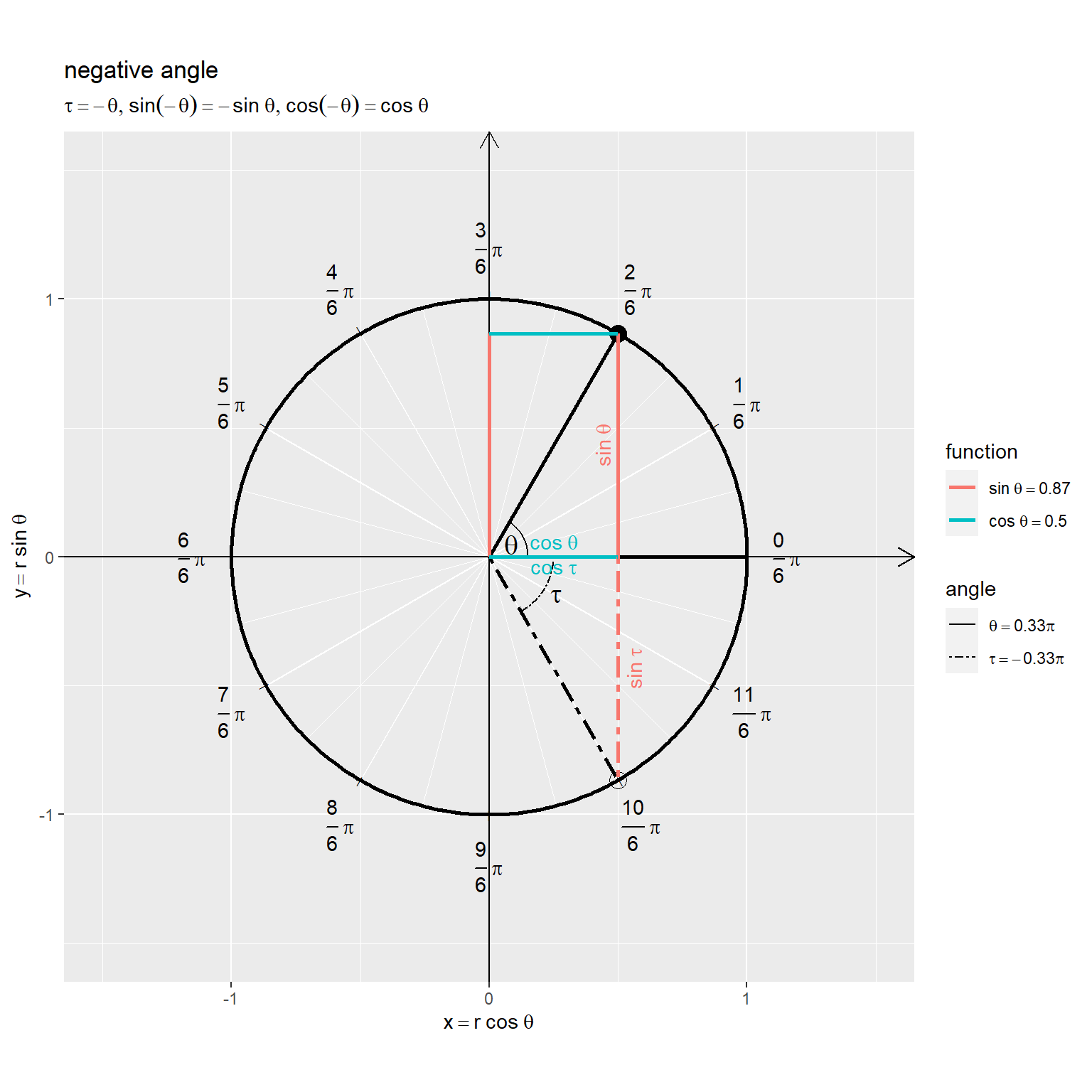
　基準となる偏角 $\theta$ を黒色の丸印と実線、符号を反転した角 $-\theta$ を白抜きの丸印と鎖線で示します。

アニメーションの作成

　変数を変化させて、単位円における偏角のアニメーションを作成します。
　作図コードについては「neg_angle.R at anemptyarchive/Mathematics · GitHub」を参照してください。

・偏角と関数の関係

　偏角 $\theta$ が、大きくなるほど左に回転(反時計回り)し、小さくなるほど右に回転(時計回り)します。
　変数 $\theta$ の符号を反転すると、sin関数の符号が反転 $\sin (-\theta) = -\sin \theta$ し、cos関数の値が変わらない $\cos(-\theta) = \cos \theta$ のを確認できます。

・偏角と座標の関係

　直線 $x = 0$ に対して線対称に変化します。

　この記事では、符号の反転を確認しました。次の記事では、直角との差を確認します。

おわりに

　sinとcosやarctanとarccotなどの関係について書いたときに余角なる概念が度々登場しました。その際は言葉だけで流したのですが一通り書き終わって少し調べてみると、直角三角形における解説はあるものの単位円(一般角)における(私がなるほど思えるような)解説や図は見当たりませんでした。
　無いなら作ろうと試行錯誤したところ、負角の説明が先に要るなとこの記事が誕生しました。負角は逆回転になるみたいな話も書いておきたかった(もう書いたことがあるかもしれないけど)という事情もありました。
　しかしほぼ書き終わってから気付いて説明を加えたのですが、θ自体が負の場合も扱っているのでその場合は-θは負角じゃないわけで、タイトルが悩ましいです。「負(の符号を付けた一般)角(と円関数の関係)の可視化」と言えば内容に即しているのかもしれません。
　今回のシリーズ(偏角編?)はどれもタイトルが微妙な感じです……そんな表現に苦労した記事がいくつか続きます。

　投稿日の前日に公開されたJuice=Juiceの新MVを最後にどうぞ。