はじめに
『ゼロから作るDeep Learning 2――自然言語処理編』の初学者向け【実装】攻略ノートです。『ゼロつく2』学習の補助となるように適宜解説を加えています。本と一緒に読んでください。
本の内容を1つずつ確認しながらゆっくりと組んでいきます。
この記事は、8.3.2項「Attention付きseq2seqの学習」と8.3.3項「Attentionの可視化」の内容です。Attention付きseq2seqの学習処理を解説して、Pythonで実装します。
【前節の内容】
【他の節の内容】
【この節の内容】
8.2.3 seq2seqの実装
この節で実装したEncoderとDecoderを用いてAttention付きseq2seqを実装します。
# 8.2.3項で利用するライブラリ
import numpy as np
seq2seqの実装には、8.3節で実装したEncoder・Decoderと5.4.2.3項で実装したTime Softmax with Lossレイヤを利用します。そのため、クラス定義を再実行するか、次の方法で実装済みのクラスを読み込む必要があります。AttentionEncoderとAttentionDecoderは、「ch08」フォルダ内の「attention_seq2seq.py」ファイルに実装されています。RNNで用いるレイヤのクラスは、「common」フォルダ内の「time_layers.py」ファイルに実装されています。
# 実装済みクラスの読み込み用の設定
import sys
sys.path.append('C://Users//「ユーザー名」//Documents//・・・//deep-learning-from-scratch-2-master')

# 実装済みのレイヤを読み込み
from ch08.attention_seq2seq import AttentionEncoder # 8.3.1項
from ch08.attention_seq2seq import AttentionDecoder # 8.3.2項
from common.time_layers import TimeSoftmaxWithLoss # 5.4.2.3項
「deep-learning-from-scratch-2-master」フォルダにパスを設定しておく必要があります。
または、7.3.3項で実装したSeq2seqクラスを継承します。
・実装
Attention付きseq2seqをクラスとして実装します。7.3.3項で実装したseq2seqのEncoderとDecoderを置き換えるだけです。処理についての詳細は7.3.3項も参照してください。
# Attention付きseq2seqの実装
class AttentionSeq2seq:
    # 初期化メソッド
    def __init__(self, vocab_size, wordvec_size, hidden_size):
        # 変数の形状に関する値を取得
        V, D, H = vocab_size, wordvec_size, hidden_size

        # 各レイヤのインスタンスを作成
        self.encoder = AttentionEncoder(V, D, H)
        self.decoder = AttentionDecoder(V, D, H)
        self.softmax = TimeSoftmaxWithLoss()

        # パラメータと勾配をリストに格納
        self.params = self.encoder.params + self.decoder.params # パラメータ
        self.grads = self.encoder.grads + self.decoder.grads    # 勾配

    # 順伝播メソッド
    def forward(self, xs, ts):
        # Decoder用の入植データを作成
        decoder_xs = ts[:, :-1] # 入力データ:(最後を除く)
        decoder_ts = ts[:, 1:]  # 教師データ:(最初を除く)

        # 各レイヤの順伝播を計算
        hs = self.encoder.forward(xs)
        score = self.decoder.forward(decoder_xs, hs)
        loss = self.softmax.forward(score, decoder_ts)
        return loss

    # 逆伝播メソッド
    def backward(self, dout=1):
        # 各レイヤの逆伝播を逆順に計算
        dout = self.softmax.backward(dout) # スコアの勾配
        dhs = self.decoder.backward(dout) # Encoderの隠れ状態の勾配
        dout = self.encoder.backward(dhs) # 出力はNone
        return dout

    # 文章生成メソッド
    def generate(self, xs, start_id, sample_size):
        # 問題文をエンコード
        hs = self.encoder.forward(xs)

        # 解答を生成
        sampled = self.decoder.generate(hs, start_id, sample_size)
        return sampled
処理上は問題はありませんが、これまでの数式上の表記と変数名を合わせるために、Encoderの順伝播の出力をhs、Decoderの逆伝播の出力をdhsに変更しました。(本当はdoutも変更したいんですけど、やっぱり本のコードと同じままの方が分かりやすいですよね?)
実装したクラスを試してみましょう。
データとパラメータの形状に関する値を設定して、seq2seqのインスタンスを作成します。
# データとパラメータの形状に関する値を指定
N = 3 # バッチサイズ(入力する文章数)
V = 10 # 単語の種類数
D = 5 # 単語ベクトルの次元数(Embedレイヤの中間層のニューロン数)
T_enc = 6 # Encoderの時系列サイズ(入力する単語数)
T_dec = 4 # Decoderの時系列サイズ(入力・予測する単語数)
H = 7 # 隠れ状態のサイズ(LSTMレイヤの中間層のニューロン数)

# seq2seqのインスタンスを作成
model = AttentionSeq2seq(V, D, H)
入力データと教師データを簡易的に作成します。
# (簡易的に)入力データを作成
xs = np.random.randint(low=0, high=V, size=(N, T_enc))
print(xs)
print(xs.shape)

# (簡易的に)教師データを作成
ts = np.random.randint(low=0, high=V, size=(N, T_dec + 1))
print(ts)
print(ts.shape)
[[4 7 5 0 2 7]
 [3 7 9 3 1 7]
 [8 3 5 1 0 2]]
(3, 6)
[[6 6 2 2 8]
 [5 6 5 5 4]
 [4 8 6 6 3]]
(3, 5)
順伝播と逆伝播を計算します。
# 順伝播を計算
loss = model.forward(xs, ts)
print(loss)

# 逆伝播を計算
dout = model.backward(dout=1)
print(dout)
2.3023338317871094
None
順伝播メソッドを実行すると損失を返します。逆伝播メソッドを実行すると何も返さず、インスタンス内で各レイヤのパラメータの勾配が保存されます。
以上でAttention付きseq2seqを実装できました。次節では、Attention付きseq2seqを使って学習を行います。
8.3.2 Attention付きseq2seqの学習
日付データセットを用いて、Attention付きseq2seqの学習を行います。学習処理は、7.3.4項と同様に行えます。
学習に用いる実装済みのクラスを読み込みます。
# 8.3.2項で利用するライブラリ
import numpy as np
import matplotlib.pyplot as plt

# 実装済みクラスの読み込み用の設定
import sys
sys.path.append('C://Users//「ユーザー名」//Documents//・・・//deep-learning-from-scratch-2-master')

# 実装済みのクラスを読み込み
from common.optimizer import Adam # 最適化手法
from common.trainer import Trainer # 学習処理:1.4.4項
・データセットの読み込み
日付データセットを読み込みます。
# データセット読み込み用のモジュール
from dataset import sequence

# データセットの読み込み
(x_train, t_train), (x_test, t_test) = sequence.load_data('date.txt')
print(x_train.shape)
print(t_train.shape)
print(x_test.shape)
print(t_test.shape)

# 文字と文字IDの変換用ディクショナリ変数の読み込み
char_to_id, id_to_char = sequence.get_vocab()
print(len(char_to_id))
(45000, 29)
(45000, 11)
(5000, 29)
(5000, 11)
59
訓練データが4万5千個、テストデータが5千個です。59種類の文字で構成されています。
文字と文字IDは次のように対応しています。
# 文字と文字IDの変換用ディクショナリ変数を確認
print(char_to_id)
print(id_to_char)
{'s': 0, 'e': 1, 'p': 2, 't': 3, 'm': 4, 'b': 5, 'r': 6, ' ': 7, '2': 8, '7': 9, ',': 10, '1': 11, '9': 12, '4': 13, '_': 14, '-': 15, '0': 16, 'A': 17, 'u': 18, 'g': 19, '3': 20, '8': 21, '/': 22, 'T': 23, 'U': 24, 'E': 25, 'S': 26, 'D': 27, 'Y': 28, 'P': 29, 'M': 30, 'B': 31, 'R': 32, '5': 33, 'J': 34, 'N': 35, '6': 36, 'a': 37, 'i': 38, 'l': 39, 'O': 40, 'c': 41, 'o': 42, 'G': 43, 'F': 44, 'y': 45, 'n': 46, 'C': 47, 'W': 48, 'd': 49, 'I': 50, 'L': 51, 'j': 52, 'H': 53, 'v': 54, 'h': 55, 'V': 56, 'f': 57, 'w': 58}
{0: 's', 1: 'e', 2: 'p', 3: 't', 4: 'm', 5: 'b', 6: 'r', 7: ' ', 8: '2', 9: '7', 10: ',', 11: '1', 12: '9', 13: '4', 14: '_', 15: '-', 16: '0', 17: 'A', 18: 'u', 19: 'g', 20: '3', 21: '8', 22: '/', 23: 'T', 24: 'U', 25: 'E', 26: 'S', 27: 'D', 28: 'Y', 29: 'P', 30: 'M', 31: 'B', 32: 'R', 33: '5', 34: 'J', 35: 'N', 36: '6', 37: 'a', 38: 'i', 39: 'l', 40: 'O', 41: 'c', 42: 'o', 43: 'G', 44: 'F', 45: 'y', 46: 'n', 47: 'C', 48: 'W', 49: 'd', 50: 'I', 51: 'L', 52: 'j', 53: 'H', 54: 'v', 55: 'h', 56: 'V', 57: 'f', 58: 'w'}
データを確認しましょう。
# 表示するデータ番号を指定
n = 0

# 文字IDのリストを表示
print(x_train[n])
print(t_train[n])

# テキストに変換して表示
print(''.join([id_to_char[c_id] for c_id in x_train[n]]))
print(''.join([id_to_char[c_id] for c_id in t_train[n]]))
[ 8 22  9 22  9  8  7  7  7  7  7  7  7  7  7  7  7  7  7  7  7  7  7  7
  7  7  7  7  7]
[14 11 12  9  8 15 16  8 15 16  9]
2/7/72
_1972-02-07
入力する日付データは、データによって形式が異なります。
# 表示するデータ番号を指定
n = 5

# 文字IDのリストを表示
print(x_train[n])
print(t_train[n])

# テキストに変換して表示
print(''.join([id_to_char[c_id] for c_id in x_train[n]]))
print(''.join([id_to_char[c_id] for c_id in t_train[n]]))
[30 37 45  7 11 10  7 11 12  9  8  7  7  7  7  7  7  7  7  7  7  7  7  7
  7  7  7  7  7]
[14 11 12  9  8 15 16 33 15 16 11]
May 1, 1972
_1972-05-01
どの形式のデータを入力してもyyyy-mm-dd形式に変換します。
7.4.1項で行ったように、入力データを反転させて入力します。
# 入力文を反転
reverse_x_train = x_train[:, ::-1]
reverse_x_test = x_test[:, ::-1]
・学習処理
ハイパーパラメータを指定します。
# 文字の種類数(EmbedレイヤとAffineレイヤのニューロン数)を取得
vocab_size = len(char_to_id)

# 単語ベクトルのサイズ(Embedレイヤのニューロン数)を指定
wordvec_size = 16

# 隠れ状態のサイズ(LSTMレイヤのニューロン数)を指定
hidden_size = 256

# バッチサイズを指定
batch_size = 128

# エポック当たりの試行回数を指定
max_epoch = 10

# 勾配の閾値を指定
max_grad = 5.0
max_gradは、勾配クリッピングを行う際の閾値です。詳しくは6.1.4項を参照してください。
この例では、通常のseq2seq・Peeky版seq2seq・Attention付きseq2seqの学習を一度に行いましょう。モデルの学習用の用のインスタンスをそれぞれ作成します。
# Attention seq2seqのインスタンスを作成
attention_model = AttentionSeq2seq(vocab_size, wordvec_size, hidden_size)
attention_optimizer = Adam()
attention_trainer = Trainer(attention_model, attention_optimizer)

# Peeky seq2seqのインスタンスを作成
peeky_model = PeekySeq2seq(vocab_size, wordvec_size, hidden_size)
peeky_optimizer = Adam()
peeky_trainer = Trainer(peeky_model, peeky_optimizer)

# Attention seq2seqのインスタンスを作成
base_model = Seq2seq(vocab_size, wordvec_size, hidden_size)
base_optimizer = Adam()
base_trainer = Trainer(base_model, base_optimizer)
学習処理はTrainerクラスの学習メソッドfit()で行います。バッチデータの切り分けやパラメータの更新も行われます。詳しくは1.4.4項を参照してください。
1エポックごとにテストデータに対する正解率を測ります。結果をacc_listに記録します。
# 正解率の記録用のリストを初期化
attention_acc_list = []
peeky_acc_list = []
base_acc_list = []

# 繰り返し試行
for epoch in range(max_epoch):
    # 学習
    print('----- Attention seq2seq -----')
    attention_trainer.fit(reverse_x_train, t_train, max_epoch=1, batch_size=batch_size, max_grad=max_grad)
    print('----- Peeky seq2seq -----')
    peeky_trainer.fit(reverse_x_train, t_train, max_epoch=1, batch_size=batch_size, max_grad=max_grad)
    print('----- seq2seq -----')
    base_trainer.fit(reverse_x_train, t_train, max_epoch=1, batch_size=batch_size, max_grad=max_grad)

    # 正解数を初期化
    attention_correct_num = 0
    peeky_correct_num = 0
    base_correct_num = 0

    # 精度を測定
    for n in range(len(reverse_x_test)):
        # データを取得
        question = reverse_x_test[[n]]  # Encoderの入力データ(足し算の式)
        start_id = t_test[n, 0] # Decoderの入力データの最初の文字(区切り文字)
        correct = t_test[n, 1:] # 教師データ(足し算の答)

        # 解答を生成
        attention_guess = attention_model.generate(question, start_id, len(correct))
        peeky_guess = peeky_model.generate(question, start_id, len(correct))
        base_guess = base_model.generate(question, start_id, len(correct))

        # 正解数をカウント
        if attention_guess == list(correct): # 解答と正答が一致したら
            attention_correct_num += 1
        if peeky_guess == list(correct): # 解答と正答が一致したら
            peeky_correct_num += 1
        if base_guess == list(correct): # 解答と正答が一致したら
            base_correct_num += 1

    # 正解率を計算
    attention_acc = float(attention_correct_num) / len(reverse_x_test)
    attention_acc_list.append(attention_acc)
    peeky_acc = float(peeky_correct_num) / len(reverse_x_test)
    peeky_acc_list.append(peeky_acc)
    base_acc = float(base_correct_num) / len(reverse_x_test)
    base_acc_list.append(base_acc)

    # 途中経過を表示
    print('----- results -----')
    print('val attention acc:' + str(attention_acc * 100))
    print('val peeky acc:' + str(peeky_acc * 100))
    print('val base acc:' + str(base_acc * 100))
・出力(クリックで展開)
----- Attention seq2seq -----
| epoch 1 |  iter 1 / 351 | time 0[s] | loss 4.08
| epoch 1 |  iter 21 / 351 | time 11[s] | loss 3.09
| epoch 1 |  iter 41 / 351 | time 23[s] | loss 1.91
| epoch 1 |  iter 61 / 351 | time 35[s] | loss 1.73
| epoch 1 |  iter 81 / 351 | time 47[s] | loss 1.48
| epoch 1 |  iter 101 / 351 | time 59[s] | loss 1.20
| epoch 1 |  iter 121 / 351 | time 71[s] | loss 1.15
| epoch 1 |  iter 141 / 351 | time 85[s] | loss 1.10
| epoch 1 |  iter 161 / 351 | time 97[s] | loss 1.06
| epoch 1 |  iter 181 / 351 | time 109[s] | loss 1.05
| epoch 1 |  iter 201 / 351 | time 121[s] | loss 1.03
| epoch 1 |  iter 221 / 351 | time 132[s] | loss 1.03
| epoch 1 |  iter 241 / 351 | time 143[s] | loss 1.02
| epoch 1 |  iter 261 / 351 | time 155[s] | loss 1.01
| epoch 1 |  iter 281 / 351 | time 167[s] | loss 1.01
| epoch 1 |  iter 301 / 351 | time 178[s] | loss 1.00
| epoch 1 |  iter 321 / 351 | time 190[s] | loss 1.00
| epoch 1 |  iter 341 / 351 | time 202[s] | loss 0.99
----- Peeky seq2seq -----
| epoch 1 |  iter 1 / 351 | time 0[s] | loss 4.08
| epoch 1 |  iter 21 / 351 | time 6[s] | loss 2.91
| epoch 1 |  iter 41 / 351 | time 14[s] | loss 1.89
| epoch 1 |  iter 61 / 351 | time 20[s] | loss 1.78
| epoch 1 |  iter 81 / 351 | time 27[s] | loss 1.70
| epoch 1 |  iter 101 / 351 | time 34[s] | loss 1.56
| epoch 1 |  iter 121 / 351 | time 40[s] | loss 1.29
| epoch 1 |  iter 141 / 351 | time 47[s] | loss 1.15
| epoch 1 |  iter 161 / 351 | time 53[s] | loss 1.09
| epoch 1 |  iter 181 / 351 | time 60[s] | loss 1.06
| epoch 1 |  iter 201 / 351 | time 67[s] | loss 1.05
| epoch 1 |  iter 221 / 351 | time 73[s] | loss 1.04
| epoch 1 |  iter 241 / 351 | time 80[s] | loss 1.03
| epoch 1 |  iter 261 / 351 | time 86[s] | loss 1.02
| epoch 1 |  iter 281 / 351 | time 92[s] | loss 1.02
| epoch 1 |  iter 301 / 351 | time 98[s] | loss 1.01
| epoch 1 |  iter 321 / 351 | time 104[s] | loss 1.00
| epoch 1 |  iter 341 / 351 | time 110[s] | loss 0.98
----- seq2seq -----
| epoch 1 |  iter 1 / 351 | time 0[s] | loss 4.08
| epoch 1 |  iter 21 / 351 | time 5[s] | loss 3.25
| epoch 1 |  iter 41 / 351 | time 11[s] | loss 1.93
| epoch 1 |  iter 61 / 351 | time 17[s] | loss 1.78
| epoch 1 |  iter 81 / 351 | time 23[s] | loss 1.68
| epoch 1 |  iter 101 / 351 | time 28[s] | loss 1.49
| epoch 1 |  iter 121 / 351 | time 33[s] | loss 1.25
| epoch 1 |  iter 141 / 351 | time 39[s] | loss 1.17
| epoch 1 |  iter 161 / 351 | time 44[s] | loss 1.12
| epoch 1 |  iter 181 / 351 | time 50[s] | loss 1.08
| epoch 1 |  iter 201 / 351 | time 55[s] | loss 1.06
| epoch 1 |  iter 221 / 351 | time 60[s] | loss 1.05
| epoch 1 |  iter 241 / 351 | time 66[s] | loss 1.04
| epoch 1 |  iter 261 / 351 | time 72[s] | loss 1.04
| epoch 1 |  iter 281 / 351 | time 77[s] | loss 1.03
| epoch 1 |  iter 301 / 351 | time 83[s] | loss 1.02
| epoch 1 |  iter 321 / 351 | time 89[s] | loss 1.02
| epoch 1 |  iter 341 / 351 | time 96[s] | loss 1.01
----- results -----
val attention acc:0.02
val peeky acc:0.0
val base acc:0.0
(省略)
----- Attention seq2seq -----
| epoch 10 |  iter 1 / 351 | time 0[s] | loss 0.00
| epoch 10 |  iter 21 / 351 | time 9[s] | loss 0.00
| epoch 10 |  iter 41 / 351 | time 19[s] | loss 0.00
| epoch 10 |  iter 61 / 351 | time 28[s] | loss 0.00
| epoch 10 |  iter 81 / 351 | time 38[s] | loss 0.00
| epoch 10 |  iter 101 / 351 | time 47[s] | loss 0.00
| epoch 10 |  iter 121 / 351 | time 56[s] | loss 0.00
| epoch 10 |  iter 141 / 351 | time 65[s] | loss 0.00
| epoch 10 |  iter 161 / 351 | time 75[s] | loss 0.00
| epoch 10 |  iter 181 / 351 | time 84[s] | loss 0.00
| epoch 10 |  iter 201 / 351 | time 93[s] | loss 0.00
| epoch 10 |  iter 221 / 351 | time 103[s] | loss 0.00
| epoch 10 |  iter 241 / 351 | time 112[s] | loss 0.00
| epoch 10 |  iter 261 / 351 | time 121[s] | loss 0.00
| epoch 10 |  iter 281 / 351 | time 130[s] | loss 0.00
| epoch 10 |  iter 301 / 351 | time 140[s] | loss 0.00
| epoch 10 |  iter 321 / 351 | time 149[s] | loss 0.00
| epoch 10 |  iter 341 / 351 | time 158[s] | loss 0.00
----- Peeky seq2seq -----
| epoch 10 |  iter 1 / 351 | time 0[s] | loss 0.00
| epoch 10 |  iter 21 / 351 | time 5[s] | loss 0.00
| epoch 10 |  iter 41 / 351 | time 10[s] | loss 0.00
| epoch 10 |  iter 61 / 351 | time 16[s] | loss 0.00
| epoch 10 |  iter 81 / 351 | time 21[s] | loss 0.00
| epoch 10 |  iter 101 / 351 | time 26[s] | loss 0.00
| epoch 10 |  iter 121 / 351 | time 32[s] | loss 0.00
| epoch 10 |  iter 141 / 351 | time 37[s] | loss 0.00
| epoch 10 |  iter 161 / 351 | time 42[s] | loss 0.00
| epoch 10 |  iter 181 / 351 | time 48[s] | loss 0.00
| epoch 10 |  iter 201 / 351 | time 53[s] | loss 0.00
| epoch 10 |  iter 221 / 351 | time 58[s] | loss 0.00
| epoch 10 |  iter 241 / 351 | time 64[s] | loss 0.00
| epoch 10 |  iter 261 / 351 | time 69[s] | loss 0.00
| epoch 10 |  iter 281 / 351 | time 74[s] | loss 0.00
| epoch 10 |  iter 301 / 351 | time 80[s] | loss 0.00
| epoch 10 |  iter 321 / 351 | time 85[s] | loss 0.00
| epoch 10 |  iter 341 / 351 | time 90[s] | loss 0.00
----- seq2seq -----
| epoch 10 |  iter 1 / 351 | time 0[s] | loss 0.81
| epoch 10 |  iter 21 / 351 | time 5[s] | loss 0.80
| epoch 10 |  iter 41 / 351 | time 10[s] | loss 0.80
| epoch 10 |  iter 61 / 351 | time 15[s] | loss 0.80
| epoch 10 |  iter 81 / 351 | time 20[s] | loss 0.79
| epoch 10 |  iter 101 / 351 | time 25[s] | loss 0.80
| epoch 10 |  iter 121 / 351 | time 30[s] | loss 0.80
| epoch 10 |  iter 141 / 351 | time 35[s] | loss 0.80
| epoch 10 |  iter 161 / 351 | time 40[s] | loss 0.79
| epoch 10 |  iter 181 / 351 | time 45[s] | loss 0.80
| epoch 10 |  iter 201 / 351 | time 50[s] | loss 0.81
| epoch 10 |  iter 221 / 351 | time 55[s] | loss 0.80
| epoch 10 |  iter 241 / 351 | time 60[s] | loss 0.80
| epoch 10 |  iter 261 / 351 | time 65[s] | loss 0.80
| epoch 10 |  iter 281 / 351 | time 70[s] | loss 0.80
| epoch 10 |  iter 301 / 351 | time 75[s] | loss 0.80
| epoch 10 |  iter 321 / 351 | time 80[s] | loss 0.79
| epoch 10 |  iter 341 / 351 | time 86[s] | loss 0.79
----- results -----
val attention acc:100.0
val peeky acc:100.0
val base acc:0.06
3つのパターンの認識精度の推移を重ねてプロットしましょう。
# 作図
plt.figure(figsize=(9, 6))
plt.plot(1 + np.arange(len(base_acc_list)), base_acc_list,
         marker='v', label='baseline') # seq2seqの結果
plt.plot(1 + np.arange(len(peeky_acc_list)), peeky_acc_list,
         marker='D', label='peeky') # Peeky seq2seqの結果
plt.plot(1 + np.arange(len(attention_acc_list)), attention_acc_list,
         marker='o', label='attention') # Attention seq2seqの結果
plt.xlabel('epoch')
plt.ylabel('accuracy')
plt.title('seq2seq', fontsize=20)
#plt.ylim(0, 1) # y軸の表示範囲
plt.grid() # グリッド線
plt.legend()
plt.show()
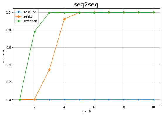
Attention付きseq2seqを利用した結果が一番早く学習できているのを確認できます。
以上でAttention付きseq2seqの実装と学習を行えました。次項では、Attentionについて確認します。
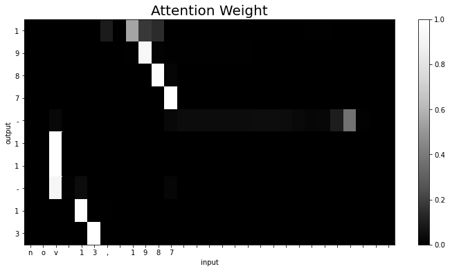
8.3.3 Attentionの可視化
学習済みのAttention付きseq2seqのAttentionの重みをヒートマップにより可視化することで、注意機構がどのように機能しているのかを確認しましょう。
データを1入力して順伝播メソッドを実行します。AttentionSeq2seqのインスタンス変数としてAttentionの重みが保存されます。
# データ番号を設定
idx = [0] # 値を指定
idx = [np.random.randint(0, len(reverse_x_test))] #ランダムに設定
print(idx)

# データを取得
x = reverse_x_test[idx]
t = t_test[idx]
print(x.shape)
print(t.shape)

# Attentionの重みを生成
attention_model.forward(x, t)

# Attentionの重みを取得
weights = attention_model.decoder.attention.attention_weights

# リストからNumPy配列に変換
weights = np.array(weights)
print(weights.shape)
[4681]
(1, 29)
(1, 11)
(10, 1, 29)
attention_weightsは、Decoderの時系列サイズ$T$(この例ではt_testの要素数-1)、バッチサイズ$N$(この例では1)、Encoderの時系列サイズ$T$(この例ではx_testの要素数)の3次元配列です。
attention_weightsを2次元のヒートマップで可視化するため、2次元配列に変換します。また軸ラベルとして表示するために、EncoderとDecoderに入力した文字IDを文字に変換します。
# 2次元配列に変換
attention_map = weights.reshape((weights.shape[0], weights.shape[2]))
print(attention_map.shape)

# 反転をされている列を戻す
attention_map = attention_map[:, ::-1]

# 軸ラベルを作成
row_labels = [id_to_char[c_id] for c_id in x[0, ::-1]] # 再反転
col_labels = [id_to_char[c_id] for c_id in t[0, 1:]]   # 区切り文字を除去
print(row_labels)
print(col_labels)
(10, 29)
['n', 'o', 'v', ' ', '1', '3', ',', ' ', '1', '9', '8', '7', ' ', ' ', ' ', ' ', ' ', ' ', ' ', ' ', ' ', ' ', ' ', ' ', ' ', ' ', ' ', ' ', ' ']
['1', '9', '8', '7', '-', '1', '1', '-', '1', '3']
Attentionの重みをヒートマップにより可視化します。
# 作図
plt.figure(figsize=(12, 6))
plt.pcolor(attention_map, cmap='Greys_r', vmin=0.0, vmax=1.0) # ヒートマップ
plt.xticks(ticks=np.arange(len(row_labels)) + 0.5, labels=row_labels) # x軸目盛
plt.yticks(ticks=np.arange(len(col_labels)) + 0.5, labels=col_labels) # y軸目盛
plt.gca().invert_yaxis() # y軸を反転
plt.xlabel('input')
plt.ylabel('output')
plt.title('Attention Weight', fontsize=20)
plt.colorbar()
plt.show()
以上で2巻の内容は完了です!
参考文献
- 斎藤康毅『ゼロから作るDeep Learning 2――自然言語処理編』オライリー・ジャパン,2018年.
おわりに
2巻かんりょーーーーーうっ!え?双方向RNN??えっと改良版RNNLMとGRUも飛ばしたんですよねぇ。3巻が終わっ(てあとPythonのことももう少し分かっ)たら1巻の記事から加筆修正していくのでその時にやります。
お疲れ様でした!