はじめに
円関数(三角関数)の定義や性質、公式などを可視化して理解しようシリーズです。
この記事では、R言語でcosine関数のグラフを作成します。
【前の内容】
【他の記事一覧】
【この記事の内容】
cos関数の定義の可視化
cos関数(余弦関数・コサイン関数・cosine function)の定義をグラフで確認します。cos関数は、円関数(circular functions)・三角関数(trigonometric functions)の1つです。
cos関数の形状(振幅・周期・位相・切片)の変化については各パラメータの記事や「cos関数の波形の可視化」を参照してください。
利用するパッケージを読み込みます。
# 利用パッケージ
library(tidyverse)
この記事では、基本的に パッケージ名::関数名() の記法を使うので、パッケージの読み込みは不要です。ただし、作図コードについてはパッケージ名を省略するので、ggplot2 を読み込む必要があります。
また、ネイティブパイプ演算子 |> を使います。magrittr パッケージのパイプ演算子 %>% に置き換えられますが、その場合は magrittr を読み込む必要があります。
曲線の形状
まずは、cos関数の曲線のグラフを作成します。
曲線の作成
・作図コード(クリックで展開)
変数の範囲を指定して、座標計算用のベクトルを作成します。
# 変数(ラジアン)の範囲を指定
theta_vec <- seq(from = -2*pi, to = 2*pi, length.out = 1001)
head(theta_vec)
[1] -6.283185 -6.270619 -6.258053 -6.245486 -6.232920 -6.220353
変数(ラジアン) の範囲を指定して、数値ベクトルを作成します。範囲を
の倍数にすると周期性を確認しやすくなります。円周率
は
pi で扱えます。
曲線の描画用のデータフレームを作成します。
# 曲線の座標を作成
curve_df <- tibble::tibble(
  t     = theta_vec,
  cos_t = cos(t),
  sin_t = sin(t)
)
curve_df
# A tibble: 1,001 × 3
       t cos_t    sin_t
   <dbl> <dbl>    <dbl>
 1 -6.28 1     2.45e-16
 2 -6.27 1.00  1.26e- 2
 3 -6.26 1.00  2.51e- 2
 4 -6.25 0.999 3.77e- 2
 5 -6.23 0.999 5.02e- 2
 6 -6.22 0.998 6.28e- 2
 7 -6.21 0.997 7.53e- 2
 8 -6.20 0.996 8.79e- 2
 9 -6.18 0.995 1.00e- 1
10 -6.17 0.994 1.13e- 1
# ℹ 991 more rows
変数 と関数
の値をデータフレームに格納します。比較用に、
の値も格納しておきます。cos関数は
cos()、sin関数は sin() で計算できます。
ラジアン軸目盛の表示用のベクトルを作成します。装飾用の処理です。
# 半周期(範囲π)における目盛数(分母の値)を指定
tick_num <- 2

# 目盛番号(分子の値)の範囲を設定
tick_min <- floor(min(theta_vec) / pi) * tick_num
tick_max <- ceiling(max(theta_vec) / pi) * tick_num

# 目盛番号(分子の値)を作成
tick_vec <- tick_min:tick_max

# 目盛位置を作成
rad_break_vec <- tick_vec/tick_num * pi

# 目盛ラベルを作成
rad_label_vec <- paste(round(rad_break_vec/pi, digits = 2), "* pi")
head(tick_vec); head(rad_break_vec); head(rad_label_vec)
[1] -4 -3 -2 -1  0  1
[1] -6.283185 -4.712389 -3.141593 -1.570796  0.000000  1.570796
[1] "-2 * pi"   "-1.5 * pi" "-1 * pi"   "-0.5 * pi" "0 * pi"    "0.5 * pi"
ラジアン に関する軸目盛ラベルを
を小数にした形で表示することにします。
は半周期(
間隔の範囲)における目盛数、
は(負の数を含む)目盛番号に対応します。
theta_vec の最小値・最大値に対して、 を
について整理した
を計算して、最小番号から最大番号までの整数を作成します。整数にするために、小数部分に関して最小値は
floor() で切り捨て、最大値は ceiling() で切り上げておきます。
作成した目盛番号に対応する目盛位置(ラジアン)を で計算します。
ラベルとして数式(ギリシャ文字や記号)を表示する場合は、expression() の記法を用います。その際に、オブジェクト(プログラム上の変数)を使う場合は、文字列として作成しておき parse() の text 引数に渡します。
cos関数のグラフを作成します。
# グラフサイズを設定
axis_y_size <- 2

# 関数曲線を作図
ggplot() +
  geom_segment(mapping = aes(x = c(-Inf, 0), y = c(0, -Inf),
                             xend = c(Inf, 0), yend = c(0, Inf)),
               arrow = arrow(length = unit(10, units = "pt"), ends = "last")) + # x・y軸線
  geom_line(data = curve_df,
            mapping = aes(x = t, y = cos_t, linetype = "cos"),
            linewidth = 1) + # cos曲線
  geom_line(data = curve_df,
            mapping = aes(x = t, y = sin_t, linetype = "sin"),
            linewidth = 1) + # sin曲線
  scale_linetype_manual(breaks = c("cos", "sin"),
                        values = c("solid", "dotted"),
                        labels = c(expression(cos~theta), expression(sin~theta)),
                        name = "function") + # 凡例表示用
  scale_x_continuous(breaks = rad_break_vec,
                     labels = parse(text = rad_label_vec)) + # ラジアン軸目盛
  guides(linetype = guide_legend(override.aes = list(linewidth = 0.5))) + # 凡例の体裁
  theme(legend.text.align = 1) + # 図の体裁
  coord_fixed(ratio = 1,
              ylim = c(-axis_y_size, axis_y_size)) + # アスペクト比
  labs(title = "cosine function",
       x = expression(theta),
       y = expression(f(theta)))

cos曲線を実線、sin曲線を点線で示します。
横軸(変数) はラジアン(弧度法の角度)、
は円周率です。
余角の関係より、 が成り立ちます。また、cos曲線を
軸の正の方向へ
動かすとsin曲線になります。この関係を式で表すと
です。
横軸方向の平行移動については「cos関数の位相の可視化」を参照してください。
次からは、単位円との関係を見ていきます。
単位円の作成
円関数の可視化に利用する単位円(unit circle)のグラフを確認します。
円の作図や度数法と弧度法(角度とラジアン)の関係については「【R】円周の作図 - からっぽのしょこ」を参照してください。
・作図コード(クリックで展開)
単位円の描画用のデータフレームを作成します。
# 円周の座標を作成
circle_df <- tibble::tibble(
  t = seq(from = 0, to = 2*pi, length.out = 361), # 1周期分のラジアン
  r = 1, # 半径
  x = r * cos(t),
  y = r * sin(t)
)
circle_df
# A tibble: 361 × 4
        t     r     x      y
    <dbl> <dbl> <dbl>  <dbl>
 1 0          1 1     0
 2 0.0175     1 1.00  0.0175
 3 0.0349     1 0.999 0.0349
 4 0.0524     1 0.999 0.0523
 5 0.0698     1 0.998 0.0698
 6 0.0873     1 0.996 0.0872
 7 0.105      1 0.995 0.105
 8 0.122      1 0.993 0.122
 9 0.140      1 0.990 0.139
10 0.157      1 0.988 0.156
# ℹ 351 more rows
1周分のラジアン を作成して、単位円の円周のx座標
とy座標
を計算します。
角度(ラジアン)目盛の描画用のデータフレームを作成します。
# 半円(範囲π)における目盛数(分母の値)を指定
tick_num <- 6

# 角度目盛の座標を作成:(補助目盛有り)
d <- 1.1
rad_tick_df <- tibble::tibble(
  # 座標用
  i     = seq(from = 0, to = 2*tick_num-0.5, by = 0.5), # 目盛番号(分子の値)
  t_deg = i/tick_num * 180, # 度数法の角度
  t_rad = i/tick_num * pi,  # 弧度法の角度(ラジアン)
  r     = 1, # 半径
  x     = r * cos(t_rad),
  y     = r * sin(t_rad),
  major_flag = i%%1 == 0, # 主・補助フラグ
  grid       = dplyr::if_else(major_flag, true = "major", false = "minor"), # 目盛カテゴリ
  # ラベル用
  deg_label  = dplyr::if_else(
    major_flag, true = paste0(round(t_deg, digits = 1), "*degree"), false = ""
  ), # 角度ラベル
  rad_label  = dplyr::if_else(
    major_flag, true = paste0("frac(", i, ", ", tick_num, ") ~ pi"), false = ""
  ), # ラジアンラベル
  label_x = d * x,
  label_y = d * y,
  a = t_deg + 90,
  h = 1 - (x * 0.5 + 0.5),
  v = 1 - (y * 0.5 + 0.5),
  tick_mark = dplyr::if_else(major_flag, true = "|", false = "") # 目盛指示線用
)
rad_tick_df
# A tibble: 24 × 16
       i t_deg t_rad     r         x     y major_flag grid  deg_label  rad_label
   <dbl> <dbl> <dbl> <dbl>     <dbl> <dbl> <lgl>      <chr> <chr>      <chr>
 1   0       0 0         1  1   e+ 0 0     TRUE       major "0*degree" "frac(0,…
 2   0.5    15 0.262     1  9.66e- 1 0.259 FALSE      minor ""         ""
 3   1      30 0.524     1  8.66e- 1 0.5   TRUE       major "30*degre… "frac(1,…
 4   1.5    45 0.785     1  7.07e- 1 0.707 FALSE      minor ""         ""
 5   2      60 1.05      1  5   e- 1 0.866 TRUE       major "60*degre… "frac(2,…
 6   2.5    75 1.31      1  2.59e- 1 0.966 FALSE      minor ""         ""
 7   3      90 1.57      1  6.12e-17 1     TRUE       major "90*degre… "frac(3,…
 8   3.5   105 1.83      1 -2.59e- 1 0.966 FALSE      minor ""         ""
 9   4     120 2.09      1 -5   e- 1 0.866 TRUE       major "120*degr… "frac(4,…
10   4.5   135 2.36      1 -7.07e- 1 0.707 FALSE      minor ""         ""
# ℹ 14 more rows
# ℹ 6 more variables: label_x <dbl>, label_y <dbl>, a <dbl>, h <dbl>, v <dbl>,
#   tick_mark <chr>
「曲線の作図」のときと同様に、目盛番号と対応するラジアンを作成して、円周上の座標とラベル用の文字列を作成します。ただし、補助目盛も作成します。主目盛と補助目盛を major_flag 列または grid 列で描き分けます。
目盛ラベル用の座標を label_x, label_y 列として、表示位置を原点からのノルム(半径) d で調整します。
単位円と角度目盛のグラフを作成します。
# グラフサイズを設定
axis_size <- 1.5

# 単位円を作図
ggplot() +
  geom_segment(data = rad_tick_df,
               mapping = aes(x = 0, y = 0, xend = x, yend = y),
               linetype = "dotted") + # 角度目盛線
  geom_text(data = rad_tick_df,
            mapping = aes(x = x, y = y, angle = a, label = tick_mark),
            size = 2) + # 角度目盛指示線
  geom_text(data = rad_tick_df,
            mapping = aes(x = label_x, y = label_y, label = deg_label, hjust = h, vjust = v),
            parse = TRUE) + # 角度目盛ラベル
  geom_path(data = circle_df,
            mapping = aes(x = x, y = y),
            linewidth = 1) + # 円周
  coord_fixed(ratio = 1,
              xlim = c(-axis_size, axis_size),
              ylim = c(-axis_size, axis_size)) + # アスペクト比
  labs(title = "unit circle",
       subtitle = expression(r == 1),
       x = expression(x == r ~ cos~theta),
       y = expression(y == r ~ sin~theta))

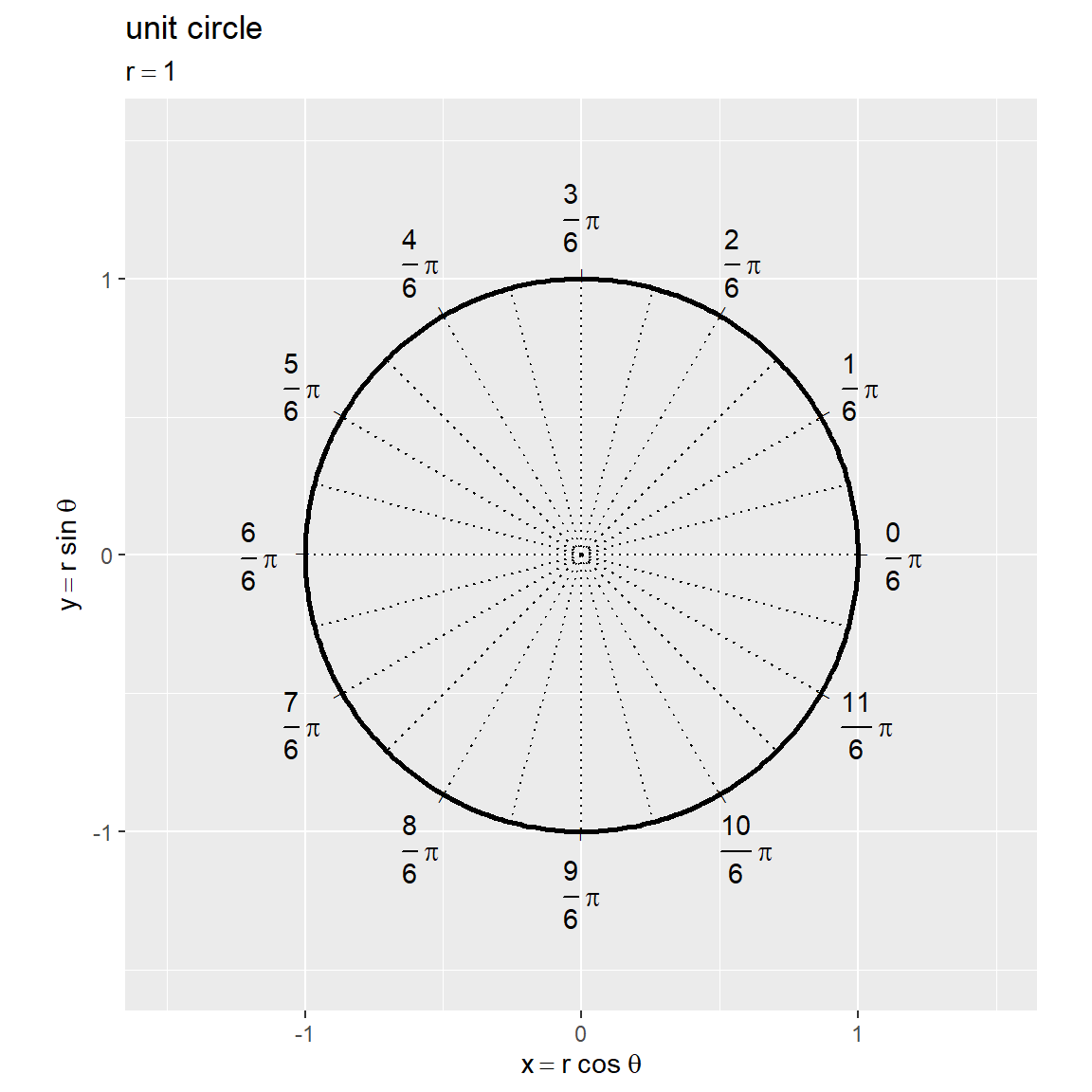
原点を中心とする半径 の円周の座標は
です。半径が
の円を単位円と呼びます。(半径や開始位置に関わらず)偏角が
(度数法だと
)で1周します。
度数法の角度 と弧度法の角度
は
の関係です。
このグラフ上に円関数の値を線分として描画します。
単位円と関数の関係
次は、単位円における偏角(単位円周上の点)と円関数(cos・sin)の関係を可視化します。
各関数についてはそれぞれの記事を参照してください。
グラフの作成
変数を固定して、単位円におけるcos関数のグラフを作成します。
・作図コード(クリックで展開)
変数を指定して、円周上の点の描画用のデータフレームを作成します。
# 点用のラジアンを指定
theta <- 1/6 * pi

# 円周上の点の座標を作成
point_df <- tibble::tibble(
  t = theta,
  x = cos(t),
  y = sin(t)
)
point_df
# A tibble: 1 × 3
      t     x     y
  <dbl> <dbl> <dbl>
1 0.524 0.866   0.5
変数 を指定して、単位円の円周上の点の座標
を計算します。
偏角を示す線分の描画用のデータフレームを作成します。
# 半径線の終点の座標を作成
radius_df <- tibble::tibble(
  x = c(1, cos(theta)),
  y = c(0, sin(theta))
)
radius_df
# A tibble: 2 × 2
      x     y
  <dbl> <dbl>
1 1       0
2 0.866   0.5
原点と点 を結ぶ線分(始線)、原点と点
を結ぶ線分(動径)用に、円周上の2点の座標を格納します。原点
の座標は、作図時に引数に直接指定します。
角マークの描画用のデータフレームを作成します。
# 角マークの座標を作成
d  <- 0.2
ds <- 0.005
angle_mark_df <- tibble::tibble(
  u = seq(from = 0, to = theta, length.out = 600),
  x = (d + ds*u) * cos(u),
  y = (d + ds*u) * sin(u)
)
angle_mark_df
# A tibble: 600 × 3
          u     x        y
      <dbl> <dbl>    <dbl>
 1 0        0.2   0
 2 0.000874 0.200 0.000175
 3 0.00175  0.200 0.000350
 4 0.00262  0.200 0.000525
 5 0.00350  0.200 0.000699
 6 0.00437  0.200 0.000874
 7 0.00524  0.200 0.00105
 8 0.00612  0.200 0.00122
 9 0.00699  0.200 0.00140
10 0.00787  0.200 0.00157
# ℹ 590 more rows
2つの線分のなす角(偏角) を示す角マークとして、
のラジアンを作成して、係数が
の螺旋の座標
を計算します。この例では、ノルムの基準値
d と間隔用の係数 ds でサイズを調整します。ds を 0 にすると、半径が の円弧の座標
になります。
角ラベルの描画用のデータフレームを作成します。
# 角ラベルの座標を計算
d <- 0.3
angle_label_df <- tibble::tibble(
  u = 0.5 * theta,
  x = d * cos(u),
  y = d * sin(u)
)
angle_label_df
# A tibble: 1 × 3
      u     x      y
  <dbl> <dbl>  <dbl>
1 0.262 0.290 0.0776
角マークの中点に角ラベルを配置することにします。 のラジアンを作成して、円弧上の点の座標を計算します。原点からのノルム
d で表示位置を調整します。
関数を示す線分の描画用のデータフレームを作成します。
# 関数の描画順を指定
fnc_level_vec <- c("cos", "sin")

# 関数線分の座標を作成
fnc_seg_df <- tibble::tibble(
  fnc = c(
    "cos", "cos",
    "sin", "sin"
  ) |>
    factor(levels = fnc_level_vec), # 関数カテゴリ
  x_from = c(
    0, 0,
    0, cos(theta)
  ),
  y_from = c(
    0, sin(theta),
    0, 0
  ),
  x_to = c(
    cos(theta), cos(theta),
    0,          cos(theta)
  ),
  y_to = c(
    0,          sin(theta),
    sin(theta), sin(theta)
  )
)
fnc_seg_df
# A tibble: 4 × 5
  fnc   x_from y_from  x_to  y_to
  <fct>  <dbl>  <dbl> <dbl> <dbl>
1 cos    0        0   0.866   0
2 cos    0        0.5 0.866   0.5
3 sin    0        0   0       0.5
4 sin    0.866    0   0.866   0.5
各線分に対応する関数カテゴリを fnc 列として線の描き分けなどに使います。線分の描画順(重なり順や色付け順)を因子レベルで設定します。
各線分の始点の座標を x_from, y_from 列、終点の座標を x_to, y_to 列として、完成図を見ながら頑張って格納します。
関数ラベルの描画用のデータフレームを作成します。
# 関数ラベルの座標を作成
fnc_label_df <- tibble::tibble(
  fnc = c("cos", "sin") |>
    factor(levels = fnc_level_vec), # 関数カテゴリ
  x = c(
    0.5 * cos(theta),
    0
  ),
  y = c(
    0,
    0.5 * sin(theta)
  ),
  fnc_label = c("cos~theta", "sin~theta"),
  a = c(0, 90),
  h = c(0.5, 0.5),
  v = c(1, -0.5)
)
fnc_label_df
# A tibble: 2 × 7
  fnc       x     y fnc_label     a     h     v
  <fct> <dbl> <dbl> <chr>     <dbl> <dbl> <dbl>
1 cos   0.433  0    cos~theta     0   0.5   1
2 sin   0      0.25 sin~theta    90   0.5  -0.5
関数ごとに1つの線分の中点に関数名を表示することにします。
ラベルの表示角度を a 列、表示角度に応じた左右の表示位置を h 列、上下の表示位置を v 列として指定します。
各種ラベルの表示用の文字列を作成します。
# ラベル用の文字列を作成
var_label <- paste0(
  "list(",
  "r == 1, ",
  "theta == ", round(theta/pi, digits = 2), " * pi",
  ")"
)
fnc_label_vec <- paste(
  c("cos~theta", "sin~theta"),
  c(cos(theta), sin(theta)) |>
    round(digits = 2),
  sep = " == "
)
var_label; fnc_label_vec
[1] "list(r == 1, theta == 0.17 * pi)"
[1] "cos~theta == 0.87" "sin~theta == 0.5"
サブタイトル用の変数ラベル、凡例用の関数ラベルを作成します。
expression() の記法では、等号は "=="、複数の(数式上の)変数は "list(変数1, 変数2)" で並べて表示できます。
単位円におけるcos関数のグラフを作成します。
# グラフサイズを設定
axis_size <- 1.5

# 単位円における関数線分を作図
ggplot() +
  geom_segment(data = rad_tick_df,
               mapping = aes(x = 0, y = 0, xend = x, yend = y, linewidth = grid),
               color = "white", show.legend = FALSE) + # θ軸目盛線
  geom_text(data = rad_tick_df,
            mapping = aes(x = x, y = y, angle = a, label = tick_mark),
            size = 2) + # θ軸目盛指示線
  geom_text(data = rad_tick_df,
            mapping = aes(x = label_x, y = label_y, label = rad_label, hjust = h, vjust = v),
            parse = TRUE) + # θ軸目盛ラベル
  geom_path(data = circle_df,
            mapping = aes(x = x, y = y),
            linewidth = 1) + # 円周
  geom_segment(data = radius_df,
               mapping = aes(x = 0, y = 0, xend = x, yend = y),
               linewidth = 1) + # 半径線
  geom_path(data = angle_mark_df,
            mapping = aes(x = x, y = y)) + # 角マーク
  geom_text(data = angle_label_df,
            mapping = aes(x = x, y = y),
            label = "theta", parse = TRUE,
            size = 5) + # 角ラベル
  geom_text(mapping = aes(x = 0.5*cos(theta+0.1), y = 0.5*sin(theta+0.1)),
            label = "r", parse = TRUE,
            size = 5) + # 半径ラベル:(θ + αで表示位置を調整)
  geom_point(data = point_df,
             mapping = aes(x = x, y = y),
             size = 4) + # 円周上の点
  geom_segment(data = fnc_seg_df,
               mapping = aes(x = x_from, y = y_from, xend = x_to, yend = y_to, color = fnc),
               linewidth = 1) + # 関数線分
  geom_text(data = fnc_label_df,
            mapping = aes(x = x, y = y, label = fnc_label, color = fnc,
                          hjust = h, vjust = v, angle = a),
            parse = TRUE, show.legend = FALSE) + # 関数ラベル
  scale_color_hue(labels = parse(text = fnc_label_vec), name = "function") + # 凡例表示用
  scale_linewidth_manual(breaks = c("major", "minor"),
                         values = c(0.5, 0.25)) + # 主・補助目盛線用
  theme(legend.text.align = 0) +
  coord_fixed(ratio = 1,
              xlim = c(-axis_size, axis_size),
              ylim = c(-axis_size, axis_size)) +
  labs(title = "circular functions",
       subtitle = parse(text = var_label),
       x = expression(x == r ~ cos~theta),
       y = expression(y == r ~ sin~theta))

偏角(始線から動径までの反時計回りの角度)を として、単位円(
の円)の円周上の点の座標は
です。
よって、cos関数の値は、単位円の円周上の点のx座標(符号付きの幅)です。
アニメーションの作成
変数を変化させて、単位円におけるcos関数のアニメーションを作成します。
作図コードについては「cos_definition.R at anemptyarchive/Mathematics · GitHub」を参照してください。
cos関数は、単位円周上の点のx座標で定義されるため、最小値が ・最大値が
で振幅が
、周期が
なのを確認できます。
単位円と曲線の関係
最後は、単位円と関数曲線のグラフを作成して、変数(ラジアン)と座標の関係を可視化します。
作図コードについては「cos_definition.R」、sin関数については「sin関数の定義の可視化」を参照してください。
変数と座標の関係
変数に応じて移動する円周上の点と曲線上の点のアニメーションを作成します。
点の座標
円周上の点とcos関数曲線上の点の関係を可視化します。
単位円におけるcos関数の値に関して、x軸の値(x軸線上の線分)を正負に応じて回転し、y軸の値(y軸線上の線分)に変換しています。
単位円周上の点のx座標と曲線上の点のy座標、円周上の点の偏角と曲線上の点のx座標が一致するのを確認できます。
円周上の点とsin関数・cos関数曲線上の点の関係を可視化します。
左下図によってx座標(横方向の線分)からy座標(縦方向の線分)に変換(回転)し、sin関数とcos関数の曲線を並べて比較します。
sin関数の値は単位円周上の点のy座標(符号付きの高さ)です。
点の推移
円周上を周回した際のcos関数の推移を可視化します。
単位円を1周する の間隔で、曲線の形状が一致するのを確認できます。
円周上を周回した際のsin関数・cos関数の推移を可視化します。
この記事では、cos関数の定義を確認しました。次の記事からは、各種パラメータによる波形への影響を確認していきます。または、tan関数の定義を確認します。
参考書籍
- 『三角関数(改定第3版)』(Newton別冊)ニュートンプレス,2022年.
おわりに
単位円に対してどこにコサイン波を置けば分かりやすいのかな、別にどこでも置けるんだな、とりあえず4つともやってみよう、で結局どれが分かりやすいんだろう、全部載せとくか。という脳内会議がありました。
まーちゃんのソロデビュー決定!!!!
#佐藤優樹 始動 pic.twitter.com/5aheCLoV8Y
— 佐藤優樹スタッフ【公式】 (@masaki_staff) 2023年1月27日
ということで、とてもめでたい。楽しみ♬
- 2023.05.10:加筆修正しました。
元々は、単位円の上・下・左上・右下にコサイン曲線を配置した4種類の図でした。4つあっても逆に分かりにくいと分かったので、再構成の必要を感じていました。他の関数の記事の構成とあわせて書き直したら、右・左・右下・左上の4種類になりました。ついでに空いてるスペースにサイン曲線も描いておきました。その他にもあれこれ図を加えました。さてこれは分かりやすいのでしょうかね。
一応その時々で自分が一番分かりやすい構成だと信じて書いているんですがね。
最後の図とか見てると、浮いたり沈んだり、近付いたり離れたり、連動してるようなしてないような、なんだかやる気曲線って感じ。
- 2024.03.20:加筆修正しました。
sin関数の記事で書いた方針で、この記事でも余分だと思われる解説を間引きました。こっちの記事の方が図が多いので、文字列ベースで文量が4分の1以下になりました。ここで省エネ化した分、各関数の変形の記事を書きたいのですが、まだ2つの関数分しか用意できていません。
今後とも浮き沈みしつつ沈没はしないようにやっていければと思います。
【次の内容】