はじめに

　円関数(三角関数)の定義や性質、公式などを可視化して理解しようシリーズです。

　この記事では、arcsin関数のグラフを作成します。

【前の内容】

www.anarchive-beta.com

【他の内容】

www.anarchive-beta.com

【この記事の内容】

はじめに
arcsin関数の定義の可視化
おわりに

arcsin関数の定義の可視化

　arcsin関数(逆sin関数・逆正弦関数・逆サイン関数・inverse sine function)の定義をグラフで確認します。arcsin関数は、逆円関数(inverse circular functions)・逆三角関数(inverse trigonometric functions)の1つです。
　sin関数の定義や作図については「【R】sin関数の可視化 - からっぽのしょこ」を参照してください。

　利用するパッケージを読み込みます。

# 利用パッケージ
library(tidyverse)

　この記事では、基本的に パッケージ名::関数名() の記法を使うので、パッケージの読み込みは不要です。ただし、作図コードについてはパッケージ名を省略するので、ggplot2 を読み込む必要があります。
　また、ネイティブパイプ演算子 |> を使います。magrittr パッケージのパイプ演算子 %>% に置き換えられますが、その場合は magrittr を読み込む必要があります。

定義式の確認

　まずは、arcsin関数の定義式を確認します。

　arcsin関数は、sin関数の逆関数で定義されます。

$\displaystyle \arcsin x = \sin^{-1} x \quad (-1 \leq x \leq 1)$

　ただし、定義域は $-1 \leq x \leq 1$ であり、終域は $-\frac{\pi}{2} \leq \arcsin x \leq \frac{\pi}{2}$ です。関数の出力はラジアン(弧度法の角度)、 $\pi$ は円周率です。

曲線の形状

　続いて、arcsin関数のグラフを作成します。

曲線の作成

・作図コード(クリックで展開)

　逆円関数の曲線の描画用のデータフレームを作成します。

# 逆関数の曲線の座標を作成
curve_inv_df <- tibble::tibble(
  x        = seq(from = -1, to = 1, length.out = 201), # 定義域内の値
  arcsin_x = asin(x), 
  arccos_x = acos(x)
)
curve_inv_df

# A tibble: 201 × 3
       x arcsin_x arccos_x
   <dbl>    <dbl>    <dbl>
 1 -1       -1.57     3.14
 2 -0.99    -1.43     3.00
 3 -0.98    -1.37     2.94
 4 -0.97    -1.33     2.90
 5 -0.96    -1.29     2.86
 6 -0.95    -1.25     2.82
 7 -0.94    -1.22     2.79
 8 -0.93    -1.19     2.77
 9 -0.92    -1.17     2.74
10 -0.91    -1.14     2.71
# ℹ 191 more rows

　変数 $-1 \leq x \leq 1$ と関数 $\arcsin x$ の値をデータフレームに格納します。比較用に、 $\arccos x$ の値も格納しておきます。arcsin関数は asin()、arccos関数は acos() で計算できます。

　円関数の曲線の描画用のデータフレームを作成します。

# 元の関数の曲線の座標を作成
curve_df <- tibble::tibble(
  t     = seq(from = -pi, to = pi, length.out = 1001), # ラジアン
  sin_t = sin(t), 
  inv_flag = (t >= -0.5*pi & t <= 0.5*pi) # 逆関数の終域
)
tmp_curve_df <- curve_df |> 
  dplyr::filter(inv_flag) # 終域内の値を抽出
curve_df

# A tibble: 1,001 × 3
       t     sin_t inv_flag
   <dbl>     <dbl> <lgl>   
 1 -3.14 -1.22e-16 FALSE   
 2 -3.14 -6.28e- 3 FALSE   
 3 -3.13 -1.26e- 2 FALSE   
 4 -3.12 -1.88e- 2 FALSE   
 5 -3.12 -2.51e- 2 FALSE   
 6 -3.11 -3.14e- 2 FALSE   
 7 -3.10 -3.77e- 2 FALSE   
 8 -3.10 -4.40e- 2 FALSE   
 9 -3.09 -5.02e- 2 FALSE   
10 -3.09 -5.65e- 2 FALSE   
# ℹ 991 more rows

　変数 $-\pi \leq \theta \leq \pi$ と関数 $\sin \theta$ の値をデータフレームに格納します。sin関数は sin() で計算できます。
　 $\theta$ の値が $\arcsin x$ のとり得る範囲内かのフラグを inv_flag 列とします。また作図の都合上、範囲内の値(行)のみのデータフレームを作成しておきます。

　arcsin関数とsin関数のグラフを作成します。

・作図コード(クリックで展開)

# ラベル用の文字列を作成
def_label <- paste0(
  "list(", 
  "arcsin~x == sin^{-1}*x, ", 
  "paste(-1 <= x, {} <= 1), ", 
  "-frac(pi, 2) <= arcsin~x <= frac(pi, 2)", 
  ")"
)

# グラフサイズを設定
axis_y_size <- 2

# 関数曲線を作図
ggplot() + 
  geom_segment(mapping = aes(x = c(-Inf, 0), y = c(0, -Inf), 
                             xend = c(Inf, 0), yend = c(0, Inf)), 
               arrow = arrow(length = unit(10, units = "pt"), ends = "last")) + # x・y軸線
  geom_line(data = curve_inv_df, 
            mapping = aes(x = x, y = arcsin_x, color = "arcsin"), 
            linewidth = 1) + # 逆関数
  geom_line(data = curve_df,
            mapping = aes(x = t, y = sin_t, color = "sin"), 
            linewidth = 1, linetype = "dotted") + # 元の関数
  geom_line(data = tmp_curve_df,
            mapping = aes(x = t, y = sin_t, color = "sin"), 
            linewidth = 1) + # 元の関数(終域内)
  geom_abline(slope = 1, intercept = 0, 
              linetype = "dotdash") + # 恒等関数
  scale_color_manual(breaks = c("arcsin", "sin"), 
                     values = c("black", "#F8766D"), 
                     labels = c(expression(arcsin~x), expression(sin~x)), 
                     name = "function") + # 凡例表示用
  coord_fixed(ratio = 1, 
              ylim = c(-axis_y_size, axis_y_size)) + # アスペクト比
  labs(title = "inverse sine function", 
       subtitle = parse(text = def_label), 
       x = expression(x), 
       y = expression(f(x)))

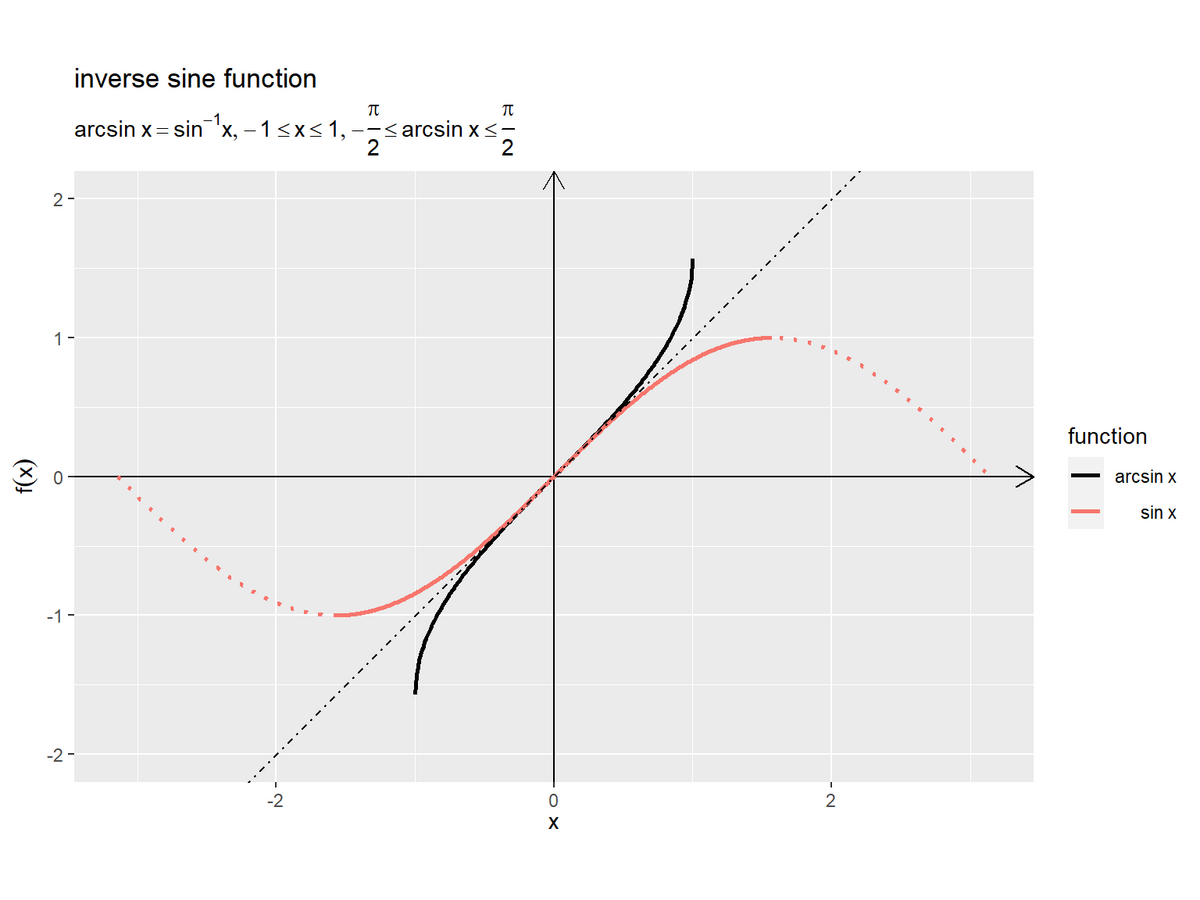
　arcsin関数を実線、sin関数を朱色の実線と点線で、また恒等関数 $f(x) = x$ を鎖線で示します。 $\tau = \arcsin x$ がとり得る範囲( $-\frac{\pi}{2} \leq \tau \leq \frac{\pi}{2}$ )の $\sin \tau$ を実線で示しています。
　恒等関数(傾きが1で切片が0の直線)に対して、arcsin曲線とsin曲線は線対称な曲線です。

　arcsin関数の軸を入れ替えたグラフを作成します。

・作図コード(クリックで展開)

# 範囲πにおける目盛数を指定
tick_num <- 2

# ラジアン軸目盛用の値を作成
rad_break_vec <- seq(from = -pi, to = pi, by = pi/tick_num)
rad_label_vec <- paste(round(rad_break_vec/pi, digits = 2), "* pi")

# グラフサイズを設定
axis_y_size <- 2

# 逆関数と元の関数の関係を作図
ggplot() + 
  geom_segment(mapping = aes(x = c(-Inf, 0), y = c(0, -Inf), 
                             xend = c(Inf, 0), yend = c(0, Inf)), 
               arrow = arrow(length = unit(10, units = "pt"), ends = "last")) + # x・y軸線
  geom_line(data = curve_inv_df, 
            mapping = aes(x = arcsin_x, y = x, color = "arcsin"), 
            linewidth = 1) + # 逆関数
  geom_line(data = curve_df,
            mapping = aes(x = t, y = sin_t, color = "sin"), 
            linewidth = 1, linetype = "dashed") + # 元の関数
  scale_color_manual(breaks = c("arcsin", "sin"), 
                     values = c("black", "#F8766D"), 
                     labels = c(expression(arcsin~x), expression(sin~theta)), 
                     name = "function") + # 凡例表示用
  scale_x_continuous(breaks = rad_break_vec, 
                     labels = parse(text = rad_label_vec)) + # ラジアン軸目盛
  coord_fixed(ratio = 1, 
              ylim = c(-axis_y_size, axis_y_size)) + # アスペクト比
  labs(title = "inverse sine function", 
       subtitle = parse(text = def_label), 
       x = expression(list(theta, tau == arcsin~x)), 
       y = expression(x == sin~theta == sin~tau))

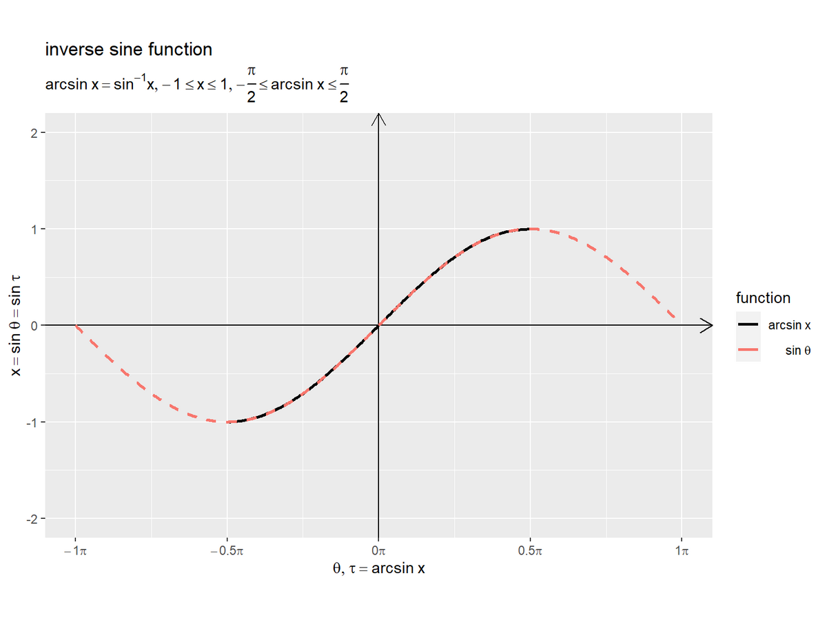
　arcsin曲線の横軸と縦軸を入れ替える(恒等関数の直線に対して反転する)と、sin曲線に一致します。
　sin関数とarcsin関数は逆関数なので、 $x = \sin(\arcsin x)$ 、また $-\frac{\pi}{2} \leq \theta \leq \frac{\pi}{2}$ のとき $\theta = \arcsin(\sin \theta)$ が成り立ちます。

　arcsin関数とarccos関数のグラフを作成します。

・作図コード(クリックで展開)

# ラベル用の文字列を作成
def_label <- "arcsin~x == frac(pi, 2) - arccos~x"

# グラフサイズを設定
axis_x_size <- 2

# 関数曲線を作図
ggplot() + 
  geom_segment(mapping = aes(x = c(-Inf, 0), y = c(0, -Inf), 
                             xend = c(Inf, 0), yend = c(0, Inf)), 
               arrow = arrow(length = unit(10, units = "pt"), ends = "last")) + # x・y軸線
  geom_hline(yintercept = 0.5*pi, 
             linetype = "dashed") + # 余角用の水平線
  geom_line(data = curve_inv_df,
            mapping = aes(x = x, y = arcsin_x, linetype = "arcsin"), 
            linewidth = 1) + # arcsin関数
  geom_line(data = curve_inv_df, 
            mapping = aes(x = x, y = arccos_x, linetype = "arccos"), 
            linewidth = 1) + # arccos関数
  scale_linetype_manual(breaks = c("arcsin", "arccos"), 
                        values = c("solid", "dotted"), 
                        labels = c(expression(arcsin~x), expression(arccos~x)), 
                        name = "function") + # 凡例表示用
  scale_y_continuous(breaks = rad_break_vec, 
                     labels = parse(text = rad_label_vec)) + # ラジアン軸目盛
  guides(linetype = guide_legend(override.aes = list(linewidth = 0.5))) + # 凡例の体裁
  coord_fixed(ratio = 1, 
              xlim = c(-axis_x_size, axis_x_size), 
              ylim = c(-pi, pi)) + # アスペクト比
  labs(title = "inverse sine function", 
       subtitle = parse(text = def_label), 
       x = expression(x), 
       y = expression(theta == f(x)))

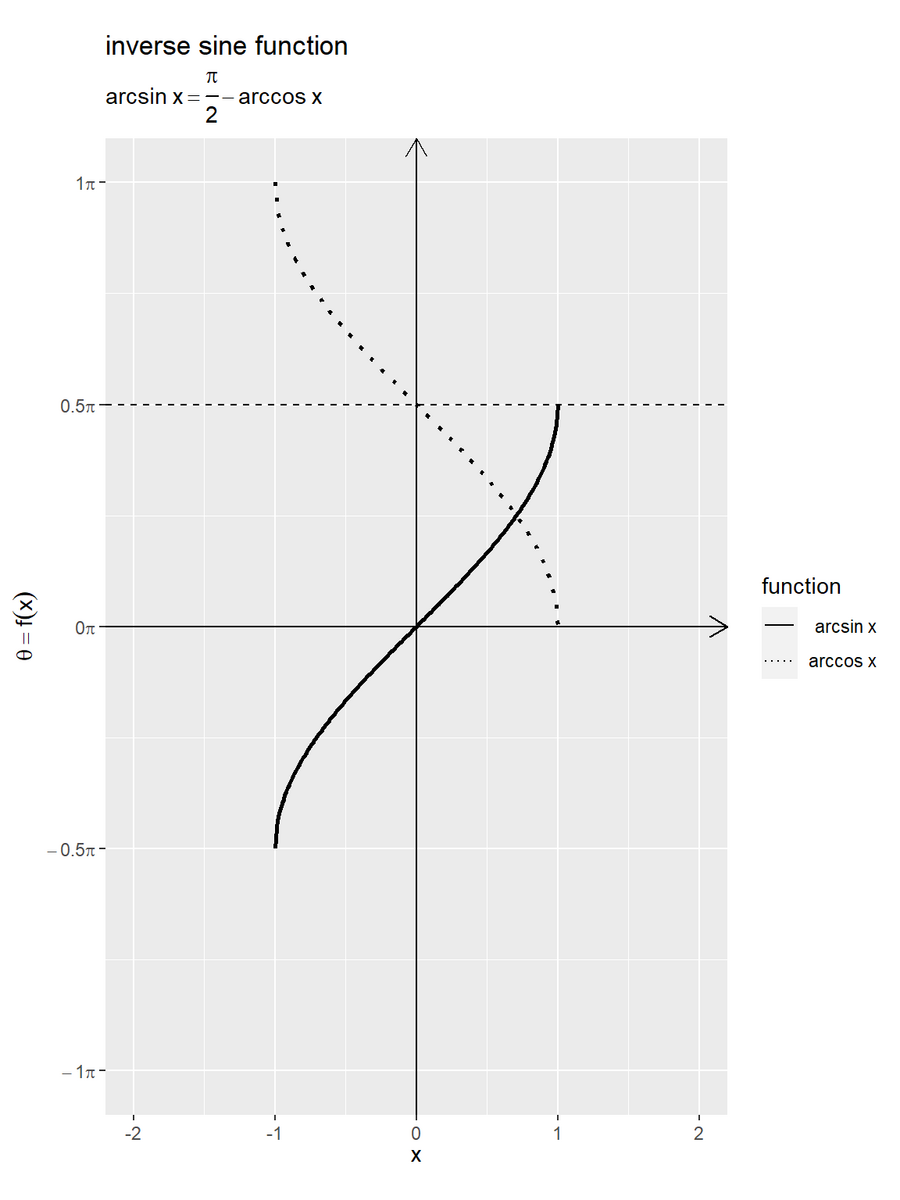
　余角の関係より、 $\arcsin x = \frac{\pi}{2} - \arccos x$ が成り立ちます。

単位円と関数の関係

　次は、単位円における偏角(単位円上の点)と円関数(sin・cos)と逆円関数(arcsin)の関係を確認します。
　各関数についてはそれぞれの記事を参照してください。

グラフの作成

　変数を固定して、単位円におけるsin関数の線分とarcsin関数の円弧のグラフを作成します。

・作図コード(クリックで展開)

　円関数の変数を指定して、逆円関数を計算します。

# 点用のラジアンを指定
theta <- 4/6 * pi

# 終域内のラジアンに変換
tau <- asin(sin(theta))
tau / pi

[1] 0.3333333

　sin関数の変数 $\theta$ を指定して、 $z = \sin \theta$ を変数としてarcsin関数 $\tau = \arcsin z$ を計算します。

　円周上の点の描画用のデータフレームを作成します。

# 円周上の点の座標を作成
point_df <- tibble::tibble(
  angle = c("theta", "tau"), # 角度カテゴリ
  t = c(theta, tau), 
  x = cos(t), 
  y = sin(t), 
  point_type = c("main", "sub") # 入出力用
)
point_df

# A tibble: 2 × 5
  angle     t     x     y point_type
  <chr> <dbl> <dbl> <dbl> <chr>     
1 theta  2.09  -0.5 0.866 main      
2 tau    1.05   0.5 0.866 sub

　円関数の入力 $\theta$ と逆円関数の出力 $\tau$ それぞれについて、単位円上の点の座標 $(x, y) = (\cos t, \sin t)$ を計算します。

　単位円の描画用のデータフレームを作成します。

# 単位円の座標を作成
circle_df <- tibble::tibble(
  t = seq(from = 0, to = 2*pi, length.out = 361), # 1周期分のラジアン
  r = 1, # 半径
  x = r * cos(t), 
  y = r * sin(t)
)

# 範囲πにおける目盛数を指定
tick_num <- 6

# 角度目盛の座標を作成
rad_tick_df <- tibble::tibble(
  i = seq(from = 0, to = 2*tick_num-0.5, by = 0.5), # 目盛番号
  t = i/tick_num * pi, # ラジアン
  r = 1, # 半径
  x = r * cos(t), 
  y = r * sin(t), 
  major_flag = i%%1 == 0, # 主・補助フラグ
  grid       = dplyr::if_else(major_flag, true = "major", false = "minor") # 目盛カテゴリ
)

　円周と角度軸目盛の座標を作成します。

　偏角の描画用のデータフレームを作成します。

# 半径線の終点の座標を作成
radius_df <- dplyr::bind_rows(
  # 始線
  tibble::tibble(
    x = 1, 
    y = 0, 
    line_type = "main" # 入出力用
  ), 
  # 動径
  point_df |> 
    dplyr::select(x, y, line_type = point_type)
)

# 角マークの座標を作成
d_in  <- 0.2
d_spi <- 0.005
d_out <- 0.3
angle_mark_df <- dplyr::bind_rows(
  # 元の関数の入力
  tibble::tibble(
    angle = "theta", # 角度カテゴリ
    u = seq(from = 0, to = theta, length.out = 600), 
    x = (d_in + d_spi*u) * cos(u), 
    y = (d_in + d_spi*u) * sin(u)
  ), 
  # 逆関数の出力
  tibble::tibble(
    angle = "tau", # 角度カテゴリ
    u = seq(from = 0, to = tau, length.out = 600), 
    x = d_out * cos(u), 
    y = d_out * sin(u)
  )
)

# 角ラベルの座標を作成
d_in  <- 0.1
d_out <- 0.4
angle_label_df <- tibble::tibble(
  u = 0.5 * c(theta, tau), 
  x = c(d_in, d_out) * cos(u), 
  y = c(d_in, d_out) * sin(u), 
  angle_label = c("theta", "tau")
)

　 $\theta, \tau$ それぞれについて、始線と動径、角マークと角ラベルの座標を作成します。

　逆円関数を示す円弧の描画用のデータフレームを作成します。

# 関数円弧の座標を作成
radian_df <- tibble::tibble(
  u = seq(from = 0, to = tau, length.out = 600), 
  r = 1, # 半径
  x = r * cos(u), 
  y = r * sin(u)
)
radian_df

# A tibble: 600 × 4
         u     r     x       y
     <dbl> <dbl> <dbl>   <dbl>
 1 0           1  1    0      
 2 0.00175     1  1.00 0.00175
 3 0.00350     1  1.00 0.00350
 4 0.00524     1  1.00 0.00524
 5 0.00699     1  1.00 0.00699
 6 0.00874     1  1.00 0.00874
 7 0.0105      1  1.00 0.0105 
 8 0.0122      1  1.00 0.0122 
 9 0.0140      1  1.00 0.0140 
10 0.0157      1  1.00 0.0157 
# ℹ 590 more rows

　ラジアン $0 \leq u \leq \tau$ を作成して、単位円の円周上の(半径が $r = 1$ の)円弧の座標 $(x, y) = (\cos u, \sin u)$ を計算します。

　円関数を示す線分の描画用のデータフレームを作成します。

# 関数の描画順を指定
fnc_level_vec <- c("arcsin", "sin", "cos")

# 関数線分の座標を作成
fnc_seg_df <- tibble::tibble(
  fnc = c(
    "sin", "sin", 
    "cos", "cos"
  ) |> 
    factor(levels = fnc_level_vec), # 関数カテゴリ
  x_from = c(
    0, cos(theta), 
    0, 0
  ), 
  y_from = c(
    0, 0, 
    0, sin(theta)
  ), 
  x_to = c(
    0,          cos(theta), 
    cos(theta), cos(theta)
  ), 
  y_to = c(
    sin(theta), sin(theta), 
    0,          sin(theta)
  )
)
fnc_seg_df

# A tibble: 4 × 5
  fnc   x_from y_from  x_to  y_to
  <fct>  <dbl>  <dbl> <dbl> <dbl>
1 sin      0    0       0   0.866
2 sin     -0.5  0      -0.5 0.866
3 cos      0    0      -0.5 0    
4 cos      0    0.866  -0.5 0.866

　各線分に対応する関数カテゴリを fnc 列として線の描き分けなどに使います。線分の描画順(重なり順や色付け順)を因子レベルで設定します。
　各線分の始点の座標を x_from, y_from 列、終点の座標を x_to, y_to 列として、完成図を見ながら頑張って格納します。

　関数ラベルの描画用のデータフレームを作成します。

# 関数ラベルの座標を作成
fnc_label_df <- tibble::tibble(
  fnc = c("arcsin", "sin", "cos") |> 
    factor(levels = fnc_level_vec), # 関数カテゴリ
  x = c(
    cos(0.5 * tau), 
    0, 
    0.5 * cos(theta)
  ), 
  y = c(
    sin(0.5 * tau),
    0.5 * sin(theta),
    0
  ), 
  fnc_label = c("arcsin(sin~theta)", "sin~theta", "cos~theta"), 
  a = c( 0,    90,  0), 
  h = c(-0.1,  0.5, 0.5), 
  v = c( 0.5, -0.5, 1)
)
fnc_label_df

# A tibble: 3 × 7
  fnc         x     y fnc_label             a     h     v
  <fct>   <dbl> <dbl> <chr>             <dbl> <dbl> <dbl>
1 arcsin  0.866 0.5   arcsin(sin~theta)     0  -0.1   0.5
2 sin     0     0.433 sin~theta            90   0.5  -0.5
3 cos    -0.25  0     cos~theta             0   0.5   1

　関数ごとに1つの線分の中点に関数名を表示することにします。
　ラベルの表示角度を a 列、表示角度に応じた左右の表示位置を h 列、上下の表示位置を v 列として指定します。

　単位円におけるarcsin関数のグラフを作成します。

# ラベル用の文字列を作成
var_label <- paste0(
  "list(", 
  "r == 1, ", 
  "theta == ", round(theta/pi, digits = 2), " * pi, ", 
  "tau == ", round(tau/pi, digits = 2), " * pi", 
  ")"
)
fnc_label_vec <- paste(
  c("arcsin(sin~theta)", "sin~theta", "cos~theta"), 
  c(tau, sin(theta), cos(theta)) |> 
    round(digits = 2), 
  sep = " == "
)

# グラフサイズを設定
axis_size <- 1.5

# 単位円における関数線分を作図
ggplot() + 
  geom_segment(data = rad_tick_df, 
               mapping = aes(x = 0, y = 0, xend = x, yend = y, linewidth = grid), 
               color = "white", show.legend = FALSE) + # θ軸目盛線
  geom_segment(mapping = aes(x = c(-Inf, 0), y = c(0, -Inf), 
                             xend = c(Inf, 0), yend = c(0, Inf)),
               arrow = arrow(length = unit(10, units = "pt"), ends = "last")) + # x・y軸線
  geom_path(data = circle_df, 
            mapping = aes(x = x, y = y), 
            linewidth = 1) + # 円周
  geom_segment(data = radius_df, 
               mapping = aes(x = 0, y = 0, xend = x, yend = y, 
                             linewidth = line_type, linetype = line_type), 
               show.legend = FALSE) + # 半径線
  geom_path(data = angle_mark_df, 
            mapping = aes(x = x, y = y, group = angle)) + # 角マーク
  geom_text(data = angle_label_df, 
            mapping = aes(x = x, y = y, label = angle_label), 
            parse = TRUE, size = 5) + # 角ラベル
  geom_text(mapping = aes(x = 0.5*cos(theta+0.1), y = 0.5*sin(theta+0.1)), 
            label = "r", parse = TRUE, 
            size = 5) + # 半径ラベル:(θ + αで表示位置を調整)
  geom_point(data = point_df, 
             mapping = aes(x = x, y = y, shape = point_type), 
             size = 4, show.legend = FALSE) + # 円周上の点
  geom_segment(mapping = aes(x = cos(theta), y = sin(theta), 
                             xend = cos(tau), yend = sin(tau)), 
               linetype = "dotted") + # 動径間の補助線
  geom_path(data = radian_df, 
            mapping = aes(x = x, y = y), 
            color = "red", linewidth = 1) + # 関数円弧
  geom_segment(data = fnc_seg_df, 
               mapping = aes(x = x_from, y = y_from, xend = x_to, yend = y_to, color = fnc), 
               linewidth = 1) + # 関数線分
  geom_text(data = fnc_label_df,
            mapping = aes(x = x, y = y, label = fnc_label, color = fnc,
                          angle = a, hjust = h, vjust = v),
            parse = TRUE, show.legend = FALSE) + # 関数ラベル
  scale_color_manual(breaks = fnc_level_vec, 
                     values = c("red", scales::hue_pal()(n = length(fnc_level_vec)-1)), 
                     labels = parse(text = fnc_label_vec), name = "function") + # 凡例表示用, 色の共通化用
  scale_shape_manual(breaks = c("main", "sub"), 
                     values = c("circle", "circle open")) + # 入出力用
  scale_linetype_manual(breaks = c("main", "sub"), 
                        values = c("solid", "dashed")) + # 入出力用
  scale_linewidth_manual(breaks = c("main", "sub", "major", "minor"), 
                         values = c(1, 0.5, 0.5, 0.25)) + # 入出力用, 主・補助目盛線用
  theme(legend.text.align = 0) + 
  coord_fixed(ratio = 1, 
              xlim = c(-axis_size, axis_size), 
              ylim = c(-axis_size, axis_size)) + 
  labs(title = "circular functions", 
       subtitle = parse(text = var_label), 
       x = expression(x == r ~ cos~theta), 
       y = expression(y == r ~ sin~theta))

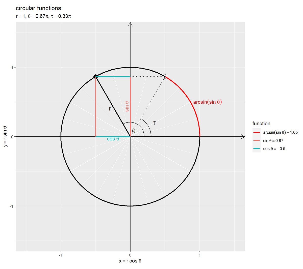
　偏角(x軸の正の部分からの角度)をラジアン $\theta$ とします。中心角が $\theta$ の弧長は $l = r \theta$ です。よって(ラジアンを用いると)、単位円における( $r = 1$ のとき)偏角 $\theta$ と弧長 $l$ が一致します。半径が $r$ の円周上の点の座標は $(x, y) = (r \cos \theta, r \sin \theta)$ です。
　sin関数の値を $z = \sin \theta$ 、arcsin関数の値を $\tau = \arcsin z$ と置く(sin関数の入力を $\theta$ 、arcsin関数の出力を $\tau$ とする)と、sin関数が $z$ になる偏角(弧長)が $\tau$ であり、 $\sin \theta = \sin \tau$ となります。

アニメーションの作成

　変数を変化させて、単位円におけるarcsin関数のアニメーションを作成します。
　作図コードについては「GitHub - anemptyarchive/Mathematics/.../arcsin_definition.R」を参照してください。

　単位円における偏角とarcsin関数の円弧の関係を可視化します。

　sin関数の終域 $-1 \leq \sin \theta \leq 1$ をarcsin関数の定義域 $-1 \leq z \leq 1$ として、終域が $-\frac{\pi}{2} \leq \arcsin z \leq \frac{\pi}{2}$ になるのを確認できます。

単位円と曲線の関係

　最後は、単位円と関数曲線のグラフを作成して、変数(ラジアン)と座標の関係を確認します。
　作図コードについては「arcsin_definition.R」を参照してください。

変数と座標の関係

　変数に応じて移動する円周上の点と曲線上の点のアニメーションを作成します。

　円周上の点とarcsin関数曲線上の点の関係を可視化します。

　 $\sin \theta$ に対応する偏角(弧長) $\tau = \arcsin(\sin \theta)$ と曲線の縦軸の値、 $z = \sin \theta = \sin \tau$ と曲線の横軸の値が一致するのを確認できます。

　この記事では、逆sin関数を確認しました。次の記事では、逆cos関数を確認します。

おわりに

　2024年の(実質)1つ目の記事です。

　円関数の可視化シリーズの派生シリーズ(螺旋編)を書いてたら、円関数シリーズの続き(波の変形編)を書きたくなって、元の記事(円関数の定義編)を読み返したらついでに書き直し始めて、なぜか逆円関数の定義編も書いてました。螺旋編の補足シリーズ(黄金比編)の記事でarctanを使う必要があったからというきっかけもあった気がします。

　これまでは、記事を書く都度アップして1年後くらいにシリーズ記事を統一的に加筆修正する運用だったのですが、短期間で修正したくなったり数年分の記事の修正待ちが溜まってきたりで、手が回らない状況です。
　これからは、シリーズ記事の類は一連の記事がひとまとめて書き上がってからアップしていくことにしました。なのでこの記事をアップした時点で、6種類の逆円関数の記事が(ほとんど)書き終わってます。円関数の修正内容も(ほとんど)書き終わってます。
　なぜこれまでしなかったかというと、書き終わっているのに上げられない状態はやきもきするんですよね。いや他の記事を書いてる間に、表現やコードの統一など微調整しまくってるので完成してないんですが。記事として上げてから修正するのは面倒が増えるし、でもさっさと上げてしまいたい。まとめて書き上がった記事を放出中に次の内容を書き上げられると、モチベ共々と上手く回せると思うのですが。

　またこれまでは、アニメーションによる可視化でgifを使っていました。はてなブログにgifを載せるのは(謎に)大変でして、今回からmp4をクラウドに上げてリンクを記事に張ることにしました。もっと良い方法もありそうですが、面倒なのでとりあえずこの方法でやってみます。
　mp4を使うことにしてブログでの動画の扱いは楽になったのですが、私のPCはmp4ファイルを作れるようにはできておらず祈りの時間(つまり待ち時間)が増えました。

　勉強の方はなんとかやれているので、今後はブログ運用の方を上手くやっていきたーい。

　2024年1月30日は、Juice=Juiceの江端妃咲さんの17歳のお誕生日です。

　(この動画ではおしとやかに話していますが)いたずらっ子で愛嬌あふれるところも見てほしいです。おめでとうございます！

【次の内容】

からっぽのしょこ

読んだら書く！書いたら読む！同じ事は二度調べ(たく)ない

【R】arcsin関数の定義の可視化

はじめに

arcsin関数の定義の可視化

定義式の確認

曲線の形状

曲線の作成

単位円と関数の関係

グラフの作成

アニメーションの作成

単位円と曲線の関係

変数と座標の関係

おわりに