はじめに

　『スタンフォード　ベクトル・行列からはじめる最適化数学』の学習ノートです。
　「数式の行間埋め」や「Pythonを使っての再現」によって理解を目指します。本と一緒に読んでください。

　この記事は7.1節「幾何変換」の内容です。
　直線に対するベクトルの鏡映の計算を確認して、グラフを作成します。

【前の内容】

www.anarchive-beta.com

【他の内容】

www.anarchive-beta.com

【今回の内容】

はじめに
ベクトルの鏡映の可視化
- ベクトルの鏡映の計算式
- ベクトルの鏡映の作図
参考書籍
おわりに

ベクトルの鏡映の可視化

　行列計算によるベクトルの直線への鏡映(vector reflection)を数式とグラフで確認します。
　行列とベクトルの積については「【Python】行列のベクトル積の可視化【『スタンフォード線形代数入門』のノート】 - からっぽのしょこ」を参照してください。

　利用するライブラリを読み込みます。

# 利用ライブラリ
import numpy as np
import matplotlib.pyplot as plt
from matplotlib.animation import FuncAnimation

ベクトルの鏡映の計算式

　まずは、ベクトルの鏡映を数式で確認します。

　 $2 \times 2$ 行列

$\displaystyle \mathbf{A} = \begin{bmatrix} \cos (2 \theta) & \sin (2 \theta) \\ \sin (2 \theta) & - \cos (2 \theta) \end{bmatrix}$

を用いて、2次元ベクトル $\mathbf{x}$ を変換します。

$\displaystyle \begin{aligned} \mathbf{y} &= \mathbf{A} \mathbf{x} \\ &= \begin{bmatrix} \cos (2 \theta) & \sin (2 \theta) \\ \sin (2 \theta) & - \cos (2 \theta) \end{bmatrix} \begin{bmatrix} x_1 \\ x_2 \end{bmatrix} \\ &= \begin{bmatrix} \cos (2 \theta) x_1 + \sin (2 \theta) x_2 \\ \sin (2 \theta) x_1 - \cos (2 \theta) x_2 \end{bmatrix} \\ &= \begin{bmatrix} y_1 \\ y_2 \end{bmatrix} \end{aligned}$

　 $\mathbf{y}$ も2次元ベクトルになります。

ベクトルの鏡映の作図

　次は、ベクトルの鏡映をグラフで確認します。

　角度を指定して、鏡映用の行列を作成します。

# 角度(ラジアン)を指定
theta = 5.0/6.0 * np.pi
print(theta) # 弧度法の角度
print(theta * 180.0/np.pi) # 度数法の角度

# 鏡映行列を作成
A = np.array(
    [[np.cos(2.0 * theta), np.sin(2.0 * theta)], 
     [np.sin(2.0 * theta), -np.cos(2.0 * theta)]]
)
print(A)
print(A.shape)

2.6179938779914944
150.00000000000003
[[ 0.5       -0.8660254]
 [-0.8660254 -0.5      ]]
(2, 2)

　水平線(x軸線の正の部分)からの角度(ラジアン) $\theta$ をスカラ theta として値を指定します。
　鏡映行列 $\mathbf{A}$ を2次元配列 A として計算します。

　ベクトルを指定して、行列との積により変換します。

# ベクトルを指定
x = np.array([-2.0, 3.0])
print(x)
print(x.shape)

# ベクトルを変換
y = np.dot(A, x)
print(y)
print(y.shape)

[-2.  3.]
(2,)
[-3.59807621  0.23205081]
(2,)

　入力ベクトル $\mathbf{x} = (x_1, x_2)^{\top}$ を1次元配列 x として値を指定します。
　鏡映ベクトル(出力ベクトル) $\mathbf{y} = \mathbf{A} \mathbf{x} = (y_1, y_2)^{\top}$ を計算して y とします。

　傾いた直線を描画するための座標を作成します。

# グラフサイズ用の値を設定
x1_min = np.floor(np.min([0.0, x[0], y[0]])) - 2
x1_max =  np.ceil(np.max([0.0, x[0], y[0]])) + 2
x2_min = np.floor(np.min([0.0, x[1], y[1]])) - 1
x2_max =  np.ceil(np.max([0.0, x[1], y[1]])) + 1

# 傾いた直線の座標を計算
x_vals = np.linspace(start=x1_min, stop=x1_max, num=101)
line_arr = np.array(
    [x_vals, 
     np.sin(theta)/np.cos(theta) * x_vals]
)
print(line_arr[:, :5])

[[-6.         -5.92       -5.84       -5.76       -5.68      ]
 [ 3.46410162  3.41791359  3.37172557  3.32553755  3.27934953]]

　原点を通り水平から $\theta$ 傾いた直線の傾きは $\frac{\sin \theta}{\cos \theta}$ で求まります。x軸の値 x_vals を作成して、y軸の値 $y = \frac{\sin \theta}{\cos \theta} x$ を計算します。

・装飾用の作図コード(クリックで展開)

　直角マークと垂線ラベルを描画するための座標を作成します。

# 傾いた直線上の単位ベクトルを作成
e_p = np.array([np.cos(theta), np.sin(theta)])
print(e_p)

# 正射影ベクトルを計算
p = np.dot(e_p, x) * e_p
print(p)

# 垂線ベクトルを計算
z = x - p
print(z)

# ベクトルを正規化
e_z = z / np.linalg.norm(z)
print(e_z)

# 直角マークの座標を計算
r = 0.2
rightangle_mark_arr = np.array(
    [[p[0]+r*e_z[0], p[0]+r*(e_z[0]-e_p[0]), p[0]-r*e_p[0]], 
     [p[1]+r*e_z[1], p[1]+r*(e_z[1]-e_p[1]), p[1]-r*e_p[1]]]
)
print(rightangle_mark_arr)

# 垂線ラベル用のラジアンを計算
sgn_p = 1.0 if p[1] >= 0.0 else -1.0
prepend_rad_val = sgn_p * np.arccos(p[0] / np.linalg.norm(p))

# 垂線ラベルの座標を計算
prepend_label_arr = np.median(
    [[x, p], [y, p]], axis=1
)
print(prepend_label_arr)

[-0.8660254  0.5      ]
[-2.79903811  1.6160254 ]
[0.79903811 1.3839746 ]
[0.5       0.8660254]
[[-2.69903811 -2.52583302 -2.62583302]
 [ 1.78923048  1.68923048  1.5160254 ]]
[[-2.39951905  2.3080127 ]
 [-3.19855716  0.92403811]]

　水平から $\theta$ 傾いた直線と平行な単位ベクトル(傾いた直線上の原点からのノルムが1の点) $\tilde{\mathbf{p}} = (\cos \theta, \sin \theta)$ を e_p として作成します。
　 $\tilde{\mathbf{p}}$ を用いて、傾いた直線に対するベクトル $\mathbf{x}$ の正射影ベクトル $\mathbf{p}$ を作成します。詳しくは「【Python】5.3：正射影ベクトルの可視化【『スタンフォード線形代数入門』のノート】 - からっぽのしょこ」を参照してください。
　点 $\mathbf{p}$ の座標から、正射影ベクトル $\mathbf{p}$ と垂線ベクトル $\mathbf{z} = \mathbf{x} - \mathbf{p}$ の方向にそれぞれ少しずつ移動した点の座標を配列に格納します。

　傾いた直線上の点 $\mathbf{p}$ と2つの点 $\mathbf{x}, \mathbf{y}$ それぞれの中点に垂線ラベルを配置します。
　 $\theta$ に応じて、ラベルの表示角度(ラジアン) prepend_rad_val を作成しておきます。

　垂線(点 $\mathbf{x}, \mathbf{y}$ を結ぶ線分)は作図時に直接指定します。

　傾きを示す角度マークと角度ラベルを描画するための座標を作成します。

# 角度マーク用のラジアンを作成
slope_rad_vals = np.linspace(start=0.0, stop=theta, num=100)

# 角度マークの座標を計算
r = 0.3
slope_mark_arr = np.array(
    [r * np.cos(slope_rad_vals), 
     r * np.sin(slope_rad_vals)]
)
print(slope_mark_arr[:, :5])

# 角度ラベルの座標を計算
r = 0.45
slope_label_vec = np.array(
    [r * np.cos(0.5 * theta), 
     r * np.sin(0.5 * theta)]
)
print(slope_label_vec)

[[0.3        0.29989511 0.29958051 0.29905643 0.29832323]
 [0.         0.00793239 0.01585923 0.02377499 0.03167412]]
[0.11646857 0.43466662]

　x軸線の正の部分(原点と点 $(1, 0)$ を結ぶ線分)から、中心角が $\theta$ の円弧の座標を計算します。円弧の中点にラベルを配置します。
　詳しくは「【Python】円周上の点とx軸を結ぶ円弧を作図したい - からっぽのしょこ」を参照してください。

　なす角を示す角度マークと角度ラベルを描画するための座標を作成します。

# 入力・出力ベクトルとx軸のなす角を計算
sgn_x   = 1.0 if x[1] >= 0.0 else -1.0
theta_x = sgn_x * np.arccos(x[0] / np.linalg.norm(x))
sgn_y   = 1.0 if y[1] >= 0.0 else -1.0
theta_y = sgn_y * np.arccos(y[0] / np.linalg.norm(y))

# 角度の差が優角なら負の角度を優角に変換
if abs(theta_x - theta_y) > np.pi:
    theta_x = theta_x if theta_x >= 0.0 else theta_x + 2.0*np.pi
    theta_y = theta_y if theta_y >= 0.0 else theta_y + 2.0*np.pi

# 角度マーク用のラジアンを作成
angle_rad_vals = np.linspace(start=theta_x, stop=theta_y, num=100)

# 角度マークの座標を計算
r = 0.6
angle_mark_arr = np.array(
    [r * np.cos(angle_rad_vals), 
     r * np.sin(angle_rad_vals)]
)
print(angle_mark_arr[:, :5])

# 角度ラベル用のラジアンを作成
theta_med = np.median(angle_rad_vals)
angle_rad_vec = np.array(
    [np.median([theta_med, theta_x]), 
     np.median([theta_med, theta_y])]
)
print(angle_rad_vec)

# 角度ラベルの座標を計算
r = 0.6
angle_label_arr = np.array(
    [r * np.cos(angle_rad_vec), 
     r * np.sin(angle_rad_vec)]
)
print(angle_label_arr)

[[-0.33282012 -0.33743692 -0.34202469 -0.34658302 -0.35111153]
 [ 0.49923018  0.49612128  0.49296969  0.48977567  0.48653951]]
[2.3883964  2.84759135]
[[-0.43770387 -0.57425522]
 [ 0.41038436  0.17387049]]

　ベクトル $\mathbf{x}, \mathbf{y}$ を結ぶ円弧の座標を計算します。傾いた直線と2つのベクトルそれぞれの中点にラベルを配置します。
　詳しくは「【Python】円周上の2点を結ぶ円弧を作図したい - からっぽのしょこ」を参照してください。

　ベクトル $\mathbf{x}, \mathbf{y}$ のグラフを作成します。

# 2D鏡映ベクトルを作図
fig, ax = plt.subplots(figsize=(8, 6), facecolor='white')
ax.quiver(0, 0, *x, 
          color='black', units='dots', width=5, headwidth=5, 
          angles='xy', scale_units='xy', scale=1, 
          label='$x=({}, {})'.format(*x)+'$') # 入力ベクトル
ax.quiver(0, 0, *y, 
          color='red', units='dots', width=5, headwidth=5, 
          angles='xy', scale_units='xy', scale=1, 
          label='$y=({:.2f}, {:.2f})'.format(*y)+'$') # 出力ベクトル
ax.plot(*line_arr) # 傾いた直線
ax.hlines(y=0.0, xmin=0.0, xmax=x1_max, linestyle='--') # 水平線
ax.plot([x[0], y[0]], [x[1], y[1]], 
        color='black', linestyle='--') # 垂線
ax.plot(*rightangle_mark_arr, 
        color='black', linewidth=1) # 直角マーク
ax.plot(*slope_mark_arr, 
        color='black', linewidth=1) # 傾き角度マーク
ax.text(*slope_label_vec, 
        s='$\\theta$', size=15, ha='center', va='center') # 傾き角度ラベル
ax.plot(*angle_mark_arr, 
        color='red', linewidth=1) # なす角マーク
for i in range(2):
    ax.annotate(xy=angle_label_arr.T[i], 
                text='|', size=10, rotation=angle_rad_vec[i]*180.0/np.pi+90.0, 
                ha='center', va='center') # なす角ラベル
    ax.annotate(xy=prepend_label_arr[i], 
                text='||', size=10, rotation=prepend_rad_val*180.0/np.pi+90.0, 
                ha='center', va='center') # 垂線ラベル
ax.set_xticks(ticks=np.arange(x1_min, x1_max+1))
ax.set_yticks(ticks=np.arange(x2_min, x2_max+1))
ax.set_xlim(left=x1_min, right=x1_max)
ax.set_ylim(bottom=x2_min, top=x2_max)
ax.set_xlabel('$x_1$')
ax.set_xlabel('$x_1$')
ax.set_ylabel('$x_2$')
ax.set_title('$y = A x, ' + 
             '\\theta = {:.2f} \pi'.format(theta/np.pi)+', ' + 
             'A = ('+', '.join(['{:.2f}'.format(a) for a in A.flatten()])+')$', loc='left')
fig.suptitle('reflection', fontsize=20)
ax.grid()
ax.legend()
ax.set_aspect('equal')
plt.show()

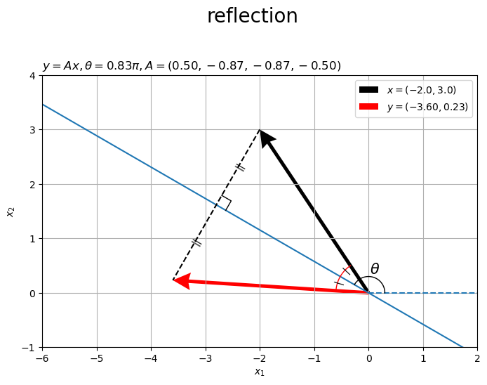
　水平(水色の破線)から反時計回りに $\theta$ 傾いた直線(水色の実線)を直線 $\theta$ と呼ぶことにします。入力ベクトル $\mathbf{x}$ を黒色の矢印、出力ベクトルを $\mathbf{y}$ を赤色の矢印で示します。
　行列 $\mathbf{A}$ によって変換したベクトル $\mathbf{y}$ が、直線 $\theta$ に対して $\mathbf{x}$ を反転させたベクトルなのが分かります。
　点 $\mathbf{x}, \mathbf{y}$ を通る直線(黒色の破線)が、直線 $\theta$ と垂直に交わります。また、直線 $\theta$ は、ベクトル $\mathbf{x}, \mathbf{y}$ のなす角、線分 $\mathbf{x}, \mathbf{y}$ それぞれの中点を通ります。

　角度(直線の傾き)または入力ベクトルを変化させたアニメーションで確認します。

・作図コード(クリックで展開)

　フレーム数を指定して、変化する角度と固定する入力ベクトルを作成します。

# フレーム数を指定
frame_num = 180

# 角度(ラジアン)の範囲を指定
theta_n = np.linspace(start=-2.0*np.pi, stop=2.0*np.pi, num=frame_num+1)[:frame_num]
print(theta_n[:5])

# ベクトルを指定
x = np.array([-2.0, 3.0])

[-6.28318531 -6.21337214 -6.14355897 -6.0737458  -6.00393263]

　フレーム数を frame_num として整数を指定します。
　ラジアンの範囲を指定して、frame_num 個のラジアン theta_n を作成します。入力ベクトル x は先ほどと同様に指定します。
　範囲を $2 n \pi$ にして frame_num + 1 個の等間隔の値を作成して最後の値を除くと、最後のフレームと最初のフレームがスムーズに繋がります。

　または、固定する角度と変化する入力ベクトルを作成します。

# フレーム数を指定
#frame_num = 90

# 角度(ラジアン)を指定
theta = 5.0/6.0 * np.pi

# ベクトルとして用いる値を指定
r = 3.0
rad_n = np.linspace(start=0.0, stop=2.0*np.pi, num=frame_num+1)[:frame_num]
x_n = np.array(
    [r * np.cos(rad_n), 
     r * np.sin(rad_n)]
).T
print(x_n[:5])

[[3.         0.        ]
 [2.99269215 0.20926942]
 [2.97080421 0.4175193 ]
 [2.9344428  0.62373507]
 [2.88378509 0.82691207]]

　frame_num 個の入力ベクトル x_nを作成します。ラジアン theta は先ほどと同様に指定します。
　この例では、入力ベクトル(の先端)が原点からの半径が r の円周上を移動するように設定しています。

　角度と入力ベクトルの両方を変化させることもできます。

　アニメーションを作成します。

# グラフサイズ用の値を設定
axis_size = np.ceil(abs(x).max()) + 1
#axis_size = np.ceil(abs(x_n).max()) + 1

# グラフオブジェクトを初期化
fig, ax = plt.subplots(figsize=(8, 8), facecolor='white')
fig.suptitle('reflection', fontsize=20)

# 作図処理を関数として定義
def update(i):
    
    # 前フレームのグラフを初期化
    plt.cla()
    
    # i番目の値を作成
    theta = theta_n[i]
    #x = x_n[i]
    
    # 鏡映行列を作成
    A = np.array(
        [[np.cos(2.0 * theta), np.sin(2.0 * theta)], 
         [np.sin(2.0 * theta), -np.cos(2.0 * theta)]]
    )
    
    # ベクトルを変換
    y = np.dot(A, x)
    
    # 傾いた直線の座標を計算
    x_vals = np.linspace(start=-axis_size, stop=axis_size, num=101)
    line_arr = np.array(
        [x_vals, 
         np.sin(theta)/np.cos(theta) * x_vals]
    )
    
    # 直角マークの座標を計算
    r = 0.3
    e_p = np.array([np.cos(theta), np.sin(theta)]) # 単位正射影ベクトル
    p   = np.dot(e_p, x) * e_p
    e_z = (x - p) / np.linalg.norm(x - p) # 単位垂線ベクトル
    rightangle_mark_arr = np.array(
        [[p[0]+r*e_z[0], p[0]+r*(e_z[0]-e_p[0]), p[0]-r*e_p[0]], 
         [p[1]+r*e_z[1], p[1]+r*(e_z[1]-e_p[1]), p[1]-r*e_p[1]]]
    )

    # 垂線ラベル用のラジアンを計算
    sgn_p = 1.0 if p[1] >= 0.0 else -1.0
    prepend_rad_val = sgn_p * np.arccos(p[0] / np.linalg.norm(p))

    # 垂線ラベルの座標を計算
    prepend_label_arr = np.median(
        [[x, p], [y, p]], axis=1
    )

    # 角度マークの座標を計算
    r = 0.3
    slope_rad_vals = np.linspace(start=0.0, stop=theta, num=100)
    slope_mark_arr = np.array(
        [r * np.cos(slope_rad_vals), 
         r * np.sin(slope_rad_vals)]
    )

    # 角度ラベルの座標を計算
    r = 0.5
    slope_label_vec = np.array(
        [r * np.cos(0.5 * theta), 
         r * np.sin(0.5 * theta)]
    )
    
    # 入力・出力ベクトルとx軸のなす角を計算
    sgn_x   = 1.0 if x[1] >= 0.0 else -1.0
    theta_x = sgn_x * np.arccos(x[0] / np.linalg.norm(x))
    sgn_y   = 1.0 if y[1] >= 0.0 else -1.0
    theta_y = sgn_y * np.arccos(y[0] / np.linalg.norm(y))
    
    # 角度の差が優角なら負の角度を優角に変換
    if abs(theta_x - theta_y) > np.pi:
        theta_x = theta_x if theta_x >= 0.0 else theta_x + 2.0*np.pi
        theta_y = theta_y if theta_y >= 0.0 else theta_y + 2.0*np.pi
    
    # 角度マークの座標を計算
    r = 0.6
    angle_rad_vals = np.linspace(start=theta_x, stop=theta_y, num=100)
    angle_mark_arr = np.array(
        [r * np.cos(angle_rad_vals), 
         r * np.sin(angle_rad_vals)]
    )
    
    # 角度ラベル用のラジアンを作成
    theta_med = np.median(angle_rad_vals)
    angle_rad_vec = np.array(
        [np.median([theta_med, theta_x]), 
         np.median([theta_med, theta_y])]
    )
    
    # 角度ラベルの座標を計算
    angle_label_arr = np.array(
        [r * np.cos(angle_rad_vec), 
         r * np.sin(angle_rad_vec)]
    )
    
    # 2D鏡映ベクトルを作図
    ax.quiver(0, 0, *x, 
              color='black', units='dots', width=5, headwidth=5, 
              angles='xy', scale_units='xy', scale=1, 
              label='$x=({: .2f}, {: .2f})'.format(*x)+'$') # 入力ベクトル
    ax.quiver(0, 0, *y, 
              color='red', units='dots', width=5, headwidth=5, 
              angles='xy', scale_units='xy', scale=1, 
              label='$y=({: .2f}, {: .2f})'.format(*y)+'$') # 出力ベクトル
    ax.plot(*line_arr) # 傾いた直線
    ax.hlines(y=0.0, xmin=0.0, xmax=axis_size, linestyle='--') # 水平線
    ax.plot([x[0], y[0]], [x[1], y[1]], 
            color='black', linestyle='--') # 垂線
    ax.plot(*rightangle_mark_arr, 
            color='black', linewidth=1) # 直角マーク
    ax.plot(*slope_mark_arr, 
            color='black', linewidth=1) # 傾き角度マーク
    ax.text(*slope_label_vec, 
            s='$\\theta$', size=15, ha='center', va='center') # 傾き角度ラベル
    ax.plot(*angle_mark_arr, 
            color='red', linewidth=1) # なす角マーク
    for i in range(2):
        ax.annotate(xy=angle_label_arr.T[i], 
                    text='|', size=10, rotation=angle_rad_vec[i]*180.0/np.pi+90.0, ha='center', va='center') # なす角ラベル
        ax.annotate(xy=prepend_label_arr[i], 
                    text='||', size=10, rotation=prepend_rad_val*180.0/np.pi+90.0, ha='center', va='center') # 垂線ラベル
    ax.set_xticks(ticks=np.arange(-axis_size, axis_size+1))
    ax.set_yticks(ticks=np.arange(-axis_size, axis_size+1))
    ax.set_xlim(left=-axis_size, right=axis_size)
    ax.set_ylim(bottom=-axis_size, top=axis_size)
    ax.set_xlabel('$x_1$')
    ax.set_ylabel('$x_2$')
    ax.set_title('$y = A x, ' + 
                 '\\theta = {: .2f} \pi, '.format(theta/np.pi)+', ' + 
                 'A = ('+', '.join(['{: .2f}'.format(a) for a in A.flatten()])+')$', loc='left')
    ax.grid()
    ax.legend(loc='upper left')
    ax.set_aspect('equal')

# gif画像を作成
ani = FuncAnimation(fig=fig, func=update, frames=frame_num, interval=100)

# gif画像を保存
ani.save('reflection.gif')