はじめに

　『スタンフォード　ベクトル・行列からはじめる最適化数学』の学習ノートです。
　「数式の行間埋め」や「Pythonを使っての再現」によって理解を目指します。本と一緒に読んでください。

　この記事は7.1節「幾何変換」の内容です。
　直線へのベクトルの射影の計算を確認して、グラフを作成します。

【前の内容】

www.anarchive-beta.com

【他の内容】

www.anarchive-beta.com

【今回の内容】

はじめに
ベクトルの射影の可視化
- ベクトルの射影の計算式
- ベクトルの射影の作図
参考書籍
おわりに

ベクトルの射影の可視化

　行列計算によるベクトルの直線への射影(vector projection)を数式とグラフで確認します。
　行列とベクトルの積については「【Python】行列のベクトル積の可視化【『スタンフォード線形代数入門』のノート】 - からっぽのしょこ」、射影については「【Python】5.3：正射影ベクトルの可視化【『スタンフォード線形代数入門』のノート】 - からっぽのしょこ」を参照してください。

　利用するライブラリを読み込みます。

# 利用ライブラリ
import numpy as np
import matplotlib.pyplot as plt
from matplotlib.animation import FuncAnimation

ベクトルの射影の計算式

　まずは、ベクトルの射影を数式で確認します。

　 $2 \times 2$ 行列

$\displaystyle \begin{aligned} \mathbf{A} &= \begin{bmatrix} \frac{1}{2} (1 + \cos (2 \theta)) & \frac{1}{2} \sin (2 \theta) \\ \frac{1}{2} \sin (2 \theta) & \frac{1}{2} (1 - \cos (2 \theta)) \end{bmatrix} \\ &= \frac{1}{2} \begin{bmatrix} 1 + \cos (2 \theta) & \sin (2 \theta) \\ \sin (2 \theta) & 1 - \cos (2 \theta) \end{bmatrix} \end{aligned}$

を用いて、2次元ベクトル $\mathbf{x}$ を変換します。

$\displaystyle \begin{aligned} \mathbf{y} &= \mathbf{A} \mathbf{x} \\ &= \frac{1}{2} \begin{bmatrix} 1 + \cos (2 \theta) & \sin (2 \theta) \\ \sin (2 \theta) & 1 - \cos (2 \theta) \end{bmatrix} \begin{bmatrix} x_1 \\ x_2 \end{bmatrix} \\ &= \begin{bmatrix} \frac{1}{2} (1 + \cos (2 \theta)) x_1 + \frac{1}{2} \sin (2 \theta) x_2 \\ \frac{1}{2} \sin (2 \theta) x_1 + \frac{1}{2} (1 - \cos (2 \theta)) x_2 \end{bmatrix} \\ &= \begin{bmatrix} y_1 \\ y_2 \end{bmatrix} \end{aligned}$

　 $\mathbf{y}$ も2次元ベクトルになります。

ベクトルの射影の作図

　次は、ベクトルの射影をグラフで確認します。

　角度を指定して、射影用の行列を作成します。

# 角度(ラジアン)を指定
theta = 1.0/6.0 * np.pi
print(theta) # 弧度法の角度
print(theta * 180.0/np.pi) # 度数法の角度

# 射影行列を作成
A = np.array(
    [[1.0 + np.cos(2.0 * theta), np.sin(2.0 * theta)], 
     [np.sin(2.0 * theta), 1.0 - np.cos(2.0 * theta)]]
)
A *= 0.5
print(A)
print(A.shape)

0.5235987755982988
29.999999999999996
[[0.75      0.4330127]
 [0.4330127 0.25     ]]
(2, 2)

　水平線(x軸線の正の部分)からの角度(ラジアン) $\theta$ をスカラ theta として値を指定します。
　射影行列 $\mathbf{A}$ を2次元配列 A として計算します。

　ベクトルを指定して、行列との積により変換します。

# ベクトルを指定
x = np.array([-3.0, 2.0])
print(x)
print(x.shape)

# ベクトルを変換
y = np.dot(A, x)
print(y)
print(y.shape)

[-3.  2.]
(2,)
[-1.3839746  -0.79903811]
(2,)

　入力ベクトル $\mathbf{x} = (x_1, x_2)^{\top}$ を1次元配列 x として値を指定します。
　射影ベクトル(出力ベクトル) $\mathbf{y} = \mathbf{A} \mathbf{x} = (y_1, y_2)^{\top}$ を計算して y とします。

　傾いた直線を描画するための座標を作成します。

# グラフサイズ用の値を設定
x1_min = np.floor(np.min([0.0, x[0], y[0]])) - 2
x1_max =  np.ceil(np.max([0.0, x[0], y[0]])) + 2
x2_min = np.floor(np.min([0.0, x[1], y[1]])) - 1
x2_max =  np.ceil(np.max([0.0, x[1], y[1]])) + 1

# 傾いた直線の座標を計算
x_vals = np.linspace(start=x1_min, stop=x1_max, num=101)
line_arr = np.array(
    [x_vals, 
     np.sin(theta)/np.cos(theta) * x_vals]
)
print(line_arr[:, :5])

[[-5.         -4.93       -4.86       -4.79       -4.72      ]
 [-2.88675135 -2.84633683 -2.80592231 -2.76550779 -2.72509327]]

　原点を通り水平から $\theta$ 傾いた直線の傾きは $\frac{\sin \theta}{\cos \theta}$ で求まります。x軸の値 x_vals を作成して、y軸の値 $y = \frac{\sin \theta}{\cos \theta} x$ を計算します。
　射影ベクトルと平行な直線になります。

・装飾用の作図コード(クリックで展開)

　直角マークを描画するための座標を作成します。

# 垂線ベクトルを計算
z = x - y
print(z)

# ベクトルを正規化
e_y = y / np.linalg.norm(y)
e_z = z / np.linalg.norm(z)
print(e_z)

# 直角マークの座標を計算
r = 0.2
rightangle_mark_arr = np.array(
    [[y[0]+r*e_z[0], y[0]+r*(e_z[0]-e_y[0]), y[0]-r*e_y[0]], 
     [y[1]+r*e_z[1], y[1]+r*(e_z[1]-e_y[1]), y[1]-r*e_y[1]]]
)
print(rightangle_mark_arr)

[-1.6160254   2.79903811]
[-0.5        0.8660254]
[[-1.4839746  -1.31076952 -1.21076952]
 [-0.62583302 -0.52583302 -0.69903811]]

　点 $\mathbf{y}$ の座標から、射影ベクトル $\mathbf{y}$ と垂線ベクトル $\mathbf{z} = \mathbf{x} - \mathbf{y}$ の方向にそれぞれ少しずつ移動した点の座標を配列に格納します。

　傾きを示す角度マークと角度ラベルを描画するための座標を作成します。

# 角度マーク用のラジアンを作成
slope_rad_vals = np.linspace(start=0.0, stop=theta, num=100)

# 角度マークの座標を計算
r = 0.3
slope_mark_arr = np.array(
    [r * np.cos(slope_rad_vals), 
     r * np.sin(slope_rad_vals)]
)
print(slope_mark_arr[:, :5])

# 角度ラベルの座標を計算
r = 0.45
slope_mark_vec = np.array(
    [r * np.cos(0.5 * theta), 
     r * np.sin(0.5 * theta)]
)
print(slope_mark_vec)

[[0.3        0.2999958  0.29998322 0.29996224 0.29993287]
 [0.         0.00158666 0.00317327 0.00475979 0.00634618]]
[0.43466662 0.11646857]

　x軸線の正の部分(原点と点 $(1, 0)$ を結ぶ線分)から、中心角が $\theta$ の円弧の座標を計算します。円弧の中点にラベルを配置します。
　詳しくは「【Python】円周上の点とx軸を結ぶ円弧を作図したい - からっぽのしょこ」を参照してください。

　ベクトル $\mathbf{x}, \mathbf{y}$ のグラフを作成します。

# 2D射影ベクトルを作図
fig, ax = plt.subplots(figsize=(8, 6), facecolor='white')
ax.quiver(0, 0, *x, 
          color='black', units='dots', width=5, headwidth=5, 
          angles='xy', scale_units='xy', scale=1, 
          label='$x=({}, {})'.format(*x)+'$') # 入力ベクトル
ax.quiver(0, 0, *y, 
          color='red', units='dots', width=5, headwidth=5, 
          angles='xy', scale_units='xy', scale=1, 
          label='$y=({:.2f}, {:.2f})'.format(*y)+'$') # 出力ベクトル
ax.plot(*line_arr) # 傾いた直線
ax.hlines(y=0.0, xmin=0.0, xmax=x1_max, linestyle='--') # 水平線
ax.plot([x[0], y[0]], [x[1], y[1]], 
        color='black', linestyle='--') # 垂線
ax.plot(*rightangle_mark_arr, 
        color='black', linewidth=1) # 直角マーク
ax.plot(*slope_mark_arr, 
        color='black', linewidth=1) # 傾き角度マーク
ax.text(*slope_mark_vec, 
        s='$\\theta$', size=15, ha='center', va='center') # 傾き角度ラベル
ax.set_xticks(ticks=np.arange(x1_min, x1_max+1))
ax.set_yticks(ticks=np.arange(x2_min, x2_max+1))
ax.set_xlim(left=x1_min, right=x1_max)
ax.set_ylim(bottom=x2_min, top=x2_max)
ax.set_xlabel('$x_1$')
ax.set_ylabel('$x_2$')
ax.set_title('$y = A x, ' + 
             '\\theta = {:.2f} \pi'.format(theta/np.pi)+', ' + 
             'A = ('+', '.join(['{:.2f}'.format(a) for a in A.flatten()])+')$', loc='left')
ax.grid()
fig.suptitle('projection', fontsize=20)
ax.legend()
ax.set_aspect('equal')
plt.show()

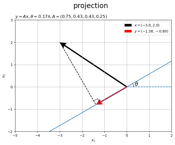
　水平(水色の破線)から反時計回りに $\theta$ 傾いた直線(水色の実線)を直線 $\theta$ と呼ぶことにします。入力ベクトル $\mathbf{x}$ を黒色の矢印、出力ベクトルを $\mathbf{y}$ を赤色の矢印で示します。
　行列 $\mathbf{A}$ によって変換したベクトル $\mathbf{y}$ が、直線 $\theta$ と平行なのが分かります。
　点 $\mathbf{x}, \mathbf{y}$ を通る直線(黒色の破線)が、直線 $\theta$ と垂直に交わります。よって、ベクトル $\mathbf{y}$ が、直線 $\theta$ に対するベクトル $\mathbf{x}$ の正射影ベクトルなのが分かります。また、点 $\mathbf{y}$ が、直線 $\theta$ 上における点 $\mathbf{x}$ からの最短の点なのが分かります。

　角度(直線の傾き)または入力ベクトルを変化させたアニメーションで確認します。

・作図コード(クリックで展開)

　フレーム数を指定して、変化する角度と固定する入力ベクトルを作成します。

# フレーム数を指定
frame_num = 180

# 角度(ラジアン)の範囲を指定
theta_n = np.linspace(start=-2.0*np.pi, stop=2.0*np.pi, num=frame_num+1)[:frame_num]
print(theta_n[:5])

# ベクトルを指定
x = np.array([-3.0, 2.0])

[-6.28318531 -6.21337214 -6.14355897 -6.0737458  -6.00393263]

　フレーム数を frame_num として整数を指定します。
　ラジアンの範囲を指定して、frame_num 個のラジアン theta_n を作成します。入力ベクトル x は先ほどと同様に指定します。
　範囲を $2 n \pi$ にして frame_num + 1 個の等間隔の値を作成して最後の値を除くと、最後のフレームと最初のフレームがスムーズに繋がります。

　または、固定する角度と変化する入力ベクトルを作成します。

# フレーム数を指定
#frame_num = 90

# 角度(ラジアン)を指定
theta = 1.0/6.0 * np.pi

# ベクトルとして用いる値を指定
r = 3.0
rad_n = np.linspace(start=0.0, stop=2.0*np.pi, num=frame_num+1)[:frame_num]
x_n = np.array(
    [r * np.cos(rad_n), 
     r * np.sin(rad_n)]
).T
print(x_n[:5])

[[3.         0.        ]
 [2.99269215 0.20926942]
 [2.97080421 0.4175193 ]
 [2.9344428  0.62373507]
 [2.88378509 0.82691207]]

　frame_num 個の入力ベクトル x_nを作成します。ラジアン theta は先ほどと同様に指定します。
　この例では、入力ベクトル(の先端)が原点からの半径が r の円周上を移動するように設定しています。

　角度と入力ベクトルの両方を変化させることもできます。

　アニメーションを作成します。

# グラフサイズ用の値を設定
axis_size = np.ceil(abs(x).max()) + 1
#axis_size = np.ceil(abs(x_n).max()) + 1

# グラフオブジェクトを初期化
fig, ax = plt.subplots(figsize=(8, 8), facecolor='white')
fig.suptitle('projection', fontsize=20)

# 作図処理を関数として定義
def update(i):
    
    # 前フレームのグラフを初期化
    plt.cla()
    
    # i番目の値を取得
    theta = theta_n[i]
    #x = x_n[i]
    
    # 射影行列を作成
    A = np.array(
        [[1.0 + np.cos(2.0*theta), np.sin(2.0*theta)], 
         [np.sin(2.0*theta), 1.0 - np.cos(2.0*theta)]]
    ) * 0.5
    
    # ベクトルを変換
    y = np.dot(A, x)
    
    # 傾いた直線の座標を計算
    x_vals = np.linspace(start=-axis_size, stop=axis_size, num=101)
    line_arr = np.array(
        [x_vals, 
         np.sin(theta)/np.cos(theta) * x_vals]
    )
    
    # 直角マークの座標を計算
    r = 0.3
    e_y = y / np.linalg.norm(y) # 単位正射影ベクトル
    e_z = (x - y) / np.linalg.norm(x - y) # 単位垂線ベクトル
    rightangle_mark_arr = np.array(
        [[y[0]+r*e_z[0], y[0]+r*(e_z[0]-e_y[0]), y[0]-r*e_y[0]], 
         [y[1]+r*e_z[1], y[1]+r*(e_z[1]-e_y[1]), y[1]-r*e_y[1]]]
    )
    
    # 角度マークの座標を計算
    r = 0.3
    slope_rad_vals = np.linspace(start=0.0, stop=theta, num=100)
    slope_mark_arr = np.array(
        [r * np.cos(slope_rad_vals), 
         r * np.sin(slope_rad_vals)]
    )

    # 角度ラベルの座標を計算
    r = 0.5
    slope_label_vec = np.array(
        [r * np.cos(0.5 * theta), 
         r * np.sin(0.5 * theta)]
    )
    
    # 2D射影ベクトルを作図
    ax.quiver(0, 0, *x, 
              color='black', units='dots', width=5, headwidth=5, 
              angles='xy', scale_units='xy', scale=1, 
              label='$x=({: .2f}, {: .2f})'.format(*x)+'$') # 入力ベクトル
    ax.quiver(0, 0, *y, 
              color='red', units='dots', width=5, headwidth=5, 
              angles='xy', scale_units='xy', scale=1, 
              label='$y=({: .2f}, {: .2f})'.format(*y)+'$') # 出力ベクトル
    ax.plot(*line_arr) # 傾いた直線
    ax.hlines(y=0.0, xmin=0.0, xmax=axis_size, linestyle='--') # 水平線
    ax.plot([x[0], y[0]], [x[1], y[1]], 
            color='black', linestyle='--') # 垂線
    ax.plot(*rightangle_mark_arr, 
            color='black', linewidth=1) # 直角マーク
    ax.plot(*slope_mark_arr, 
            color='black', linewidth=1) # 傾き角度マーク
    ax.text(*slope_label_vec, 
            s='$\\theta$', size=15, ha='center', va='center') # 傾き角度ラベル
    ax.set_xticks(ticks=np.arange(-axis_size, axis_size+1))
    ax.set_yticks(ticks=np.arange(-axis_size, axis_size+1))
    ax.set_xlim(left=-axis_size, right=axis_size)
    ax.set_ylim(bottom=-axis_size, top=axis_size)
    ax.set_xlabel('$x_1$')
    ax.set_ylabel('$x_2$')
    ax.set_title('$y = A x, ' + 
                 '\\theta = {: .2f} \pi, '.format(theta/np.pi)+', ' + 
                 'A = ('+', '.join(['{: .2f}'.format(a) for a in A.flatten()])+')$', loc='left')
    ax.grid()
    ax.legend(loc='upper left')
    ax.set_aspect('equal')

# gif画像を作成
ani = FuncAnimation(fig=fig, func=update, frames=frame_num, interval=100)

# gif画像を保存
ani.save('projection.gif')