はじめに
R言語で三角関数の定義や公式を可視化しようシリーズのスピンオフです。
この記事では、sinh関数のグラフを作成します。
【前の内容】
【他の記事一覧】
【この記事の内容】
sinh関数の可視化
双曲線関数の1つであるsinh関数(双曲線正弦関数・ハイパボリックサイン関数・hyperbolic sine function)をグラフで確認します。
利用するパッケージを読み込みます。
# 利用パッケージ
library(tidyverse)
library(patchwork)
library(gganimate)
library(magick)
この記事では、基本的にパッケージ名::関数名()の記法を使うので、パッケージを読み込む必要はありません。ただし、作図コードがごちゃごちゃしないようにパッケージ名を省略しているためggplot2を読み込む必要があります。
また、ネイティブパイプ演算子|>を使っています。magrittrパッケージのパイプ演算子%>%に置き換えても処理できますが、その場合はmagrittrも読み込む必要があります。
定義式の確認
まずは、sinh関数の定義式を確認します。
sinh関数は、次の式で定義されます。
$e^x$はネイピア数$e$を底とする自然指数関数です。
sinh関数曲線の作図
次に、sinh関数のグラフを作成します。
作図用の変数の値を作成します。
# 作図用の変数の値を指定
theta_vec <- seq(from = -5, to = 5, by = 0.01)
head(theta_vec)
## [1] -5.00 -4.99 -4.98 -4.97 -4.96 -4.95
作図に利用する変数$\theta$の範囲と間隔を指定してtheta_vecとします。
・作図コード(クリックで展開)
sinh関数の曲線を描画するためのデータフレームを作成します。
# sinh曲線の描画用
sinh_df <- tibble::tibble(
  t = theta_vec,
  sinh_t = sinh(theta_vec)
)
sinh_df
## # A tibble: 1,001 × 2
##        t sinh_t
##    <dbl>  <dbl>
##  1 -5     -74.2
##  2 -4.99  -73.5
##  3 -4.98  -72.7
##  4 -4.97  -72.0
##  5 -4.96  -71.3
##  6 -4.95  -70.6
##  7 -4.94  -69.9
##  8 -4.93  -69.2
##  9 -4.92  -68.5
## 10 -4.91  -67.8
## # … with 991 more rows
$\theta$の値と$\sinh \theta$の値をデータフレームに格納します。sinh関数はsinh()で計算できます。
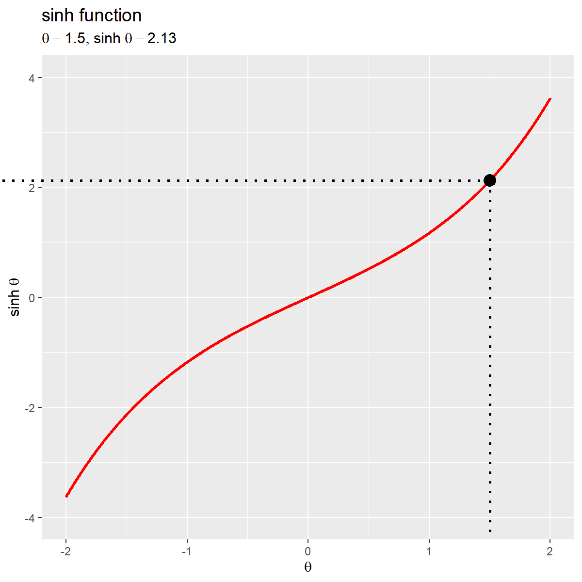
sinh関数のグラフを作成します。
# sinh関数曲線を作図
ggplot() +
  geom_line(data = sinh_df, mapping = aes(x = t, y = sinh_t),
            size = 1) + # sinh曲線
  labs(title = "sinh function",
       x = expression(theta), y = expression(sinh~theta))
x軸を$\theta$、y軸を$\sinh \theta$として、geom_line()で折れ線グラフを描画します。
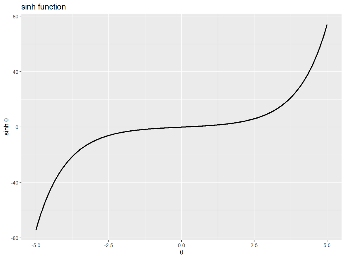
変数$\theta$の値が小さいほど$\sinh \theta$も小さく、大きいほど大きくなるのを確認できます。
双曲線の作図
続いて、sinh関数の可視化に利用する単位双曲線(unit hyperbola)のグラフを作成します。双曲線については「【R】双曲線の作図 - からっぽのしょこ」を参照してください。
・作図コード(クリックで展開)
作図に利用するデータフレームを作成します。
# 作図用の変数の値を指定
theta_vec <- seq(from = -2, to = 2, by = 0.002)

# 双曲線の描画用
hyperbola_df <- tibble::tibble(
  t = c(theta_vec, theta_vec),
  sinh_t = c(sinh(theta_vec), sinh(theta_vec)),
  cosh_t = c(cosh(theta_vec), -cosh(theta_vec)),
  sign = rep(c("plus", "minus"), each = length(theta_vec))# 符号
)

# 軸の最大値を設定
axis_max <- hyperbola_df[["cosh_t"]] |>
  max() |>
  ceiling()

# 漸近線の描画用
asymptote_df <- tibble::tibble(
  x = seq(from = -axis_max, to = axis_max, length.out = 100) |>
    rep(times = 2),
  y = rep(c(1, -1), each = 100) * x,
  slope = rep(c("plus", "minus"), each = 100) # 符号
)

# 正方形グリッドの描画用
square_df <- tibble::tibble(
  x = c(1, 1, -1, -1, 1),
  y = c(1, -1, -1, 1, 1)
)

# 軸線の描画用
axis_df <- tibble::tibble(
  x_from = c(-axis_max, 0),
  y_from = c(0, -axis_max),
  x_to = c(axis_max, 0),
  y_to = c(0, axis_max),
  axis = c("x", "y")
)
双曲線と補助線のグラフを作成します。
# 単位双曲線を作図
ggplot() +
  geom_segment(data = axis_df,
               mapping = aes(x = x_from, y = y_from, xend = x_to, yend = y_to, group = "axis"),
               arrow = arrow(length = unit(10, units = "pt"))) + # 軸線
  geom_path(data = square_df,
            mapping = aes(x = x, y = y), linetype = "dashed") + # 正方形グリッド
  geom_line(data = asymptote_df,
            mapping = aes(x = x, y = y, group = slope), linetype = "dashed") + # 漸近線
  geom_path(data = hyperbola_df,
            mapping = aes(x = cosh_t, y = sinh_t, group = sign),
            size = 1) + # 双曲線
  theme(legend.text.align = 0.5) + # 凡例の体裁:(凡例表示用)
  coord_fixed(ratio = 1,
              xlim = c(-axis_max, axis_max), ylim = c(-axis_max, axis_max)) + # 表示範囲
  labs(title = "unit hyperbola",
       x = "x", y = "y")
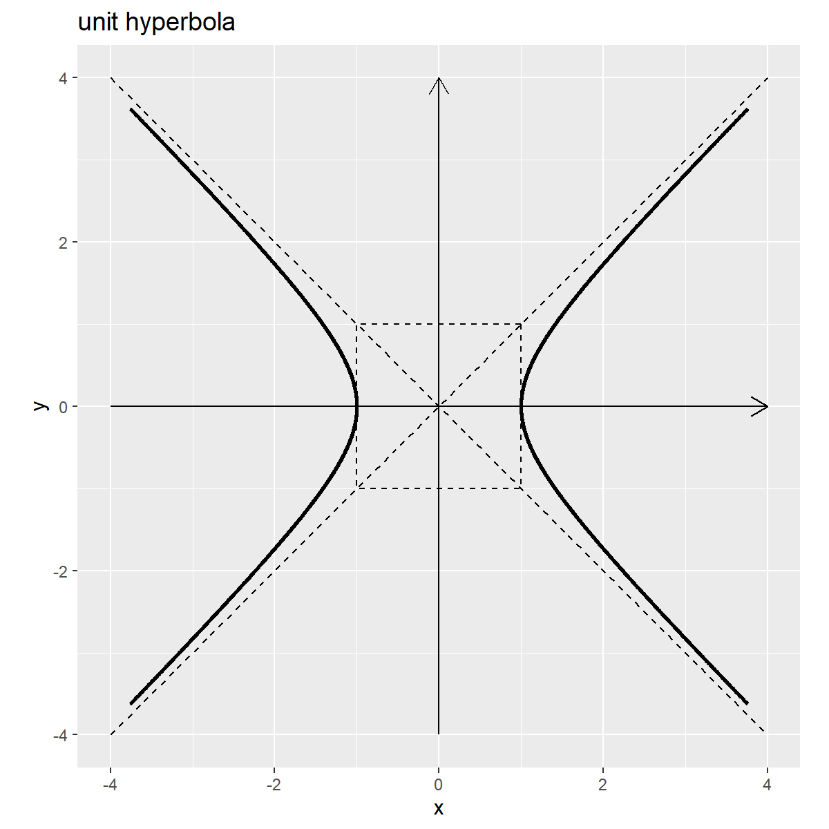
このグラフ上に双曲線関数を描画します。
双曲線上のsinh関数の可視化
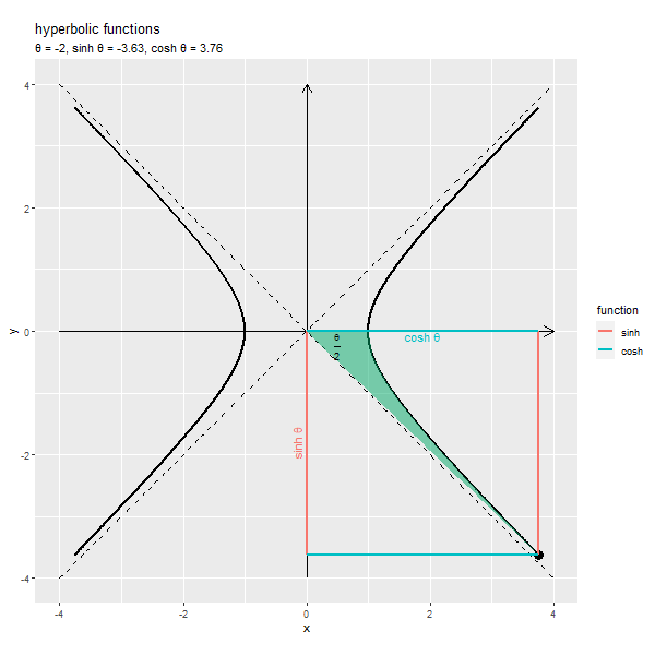
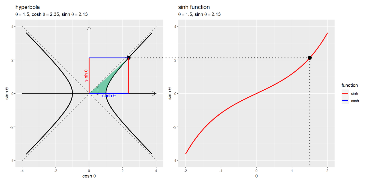
次は、単位双曲線上における双曲線関数(sinh・cosh)のグラフを作成します。
グラフの作成
変数を固定したsinh関数をグラフで確認します。
変数の値を設定します。
# 変数の値を指定
theta <- 1.5
変数$\theta$の値を指定します。
・作図コード(クリックで展開)
曲線上の点を描画するためのデータフレームを作成します。
# 曲線上の点の描画用
point_df <- tibble::tibble(
  t = theta,
  sinh_t = sinh(theta),
  cosh_t = cosh(theta)
)
point_df
## # A tibble: 1 × 3
##       t sinh_t cosh_t
##   <dbl>  <dbl>  <dbl>
## 1   1.5   2.13   2.35
sinh曲線上の点のx軸の値$\theta$とy軸の値$\sinh \theta$、単位双曲線上の点のx軸の値$\cosh \theta$とy軸の値$\sinh \theta$を格納します。
変数の値(の半分)を面積(塗りつぶし領域)として描画するためのデータフレームを作成します。
# 変数(面積)の描画用
variable_area_df <- tibble::tibble(
  x = seq(from = 0, to = cosh(theta), length.out = 50),
  sign = dplyr::if_else(theta >= 0, true = 1, false = -1), # 符号
  curve = sign * sqrt(x^2 - 1), # x軸と双曲線上の線分
  straight = sinh(theta)/cosh(theta) * x # 原点と曲線上の点の線分
) |>
  dplyr::mutate(
    curve = dplyr::if_else(is.na(curve), true = 0, false = curve)
  ) # 双曲線の範囲外を0に置換
variable_area_df
## # A tibble: 50 × 4
##         x  sign curve straight
##     <dbl> <dbl> <dbl>    <dbl>
##  1 0          1     0   0
##  2 0.0480     1     0   0.0435
##  3 0.0960     1     0   0.0869
##  4 0.144      1     0   0.130
##  5 0.192      1     0   0.174
##  6 0.240      1     0   0.217
##  7 0.288      1     0   0.261
##  8 0.336      1     0   0.304
##  9 0.384      1     0   0.348
## 10 0.432      1     0   0.391
## # … with 40 more rows
「原点と双曲線上の点を結ぶ線分」と「$0 \leq x < 1$の範囲のx軸線($y = 0$の直線)と$1 \leq x \leq \cosh \theta$の範囲の双曲線」の範囲を塗りつぶします。ただし、双曲線について、$\theta > 0$のときは$y > 0$の範囲を塗りつぶすため$y = \sqrt{x^2 - 1}$、$\theta < 0$のときは$y < 0$の範囲を塗りつぶすため$y = - \sqrt{x^2 - 1}$を使います。
x軸の値として$0$から$\cosh \theta$の範囲の値を作成してx列とします。
thetaの正負によって符号を変更してsign列としておき、双曲線を計算してcurve列とします。ただし、$0$から$1$の範囲がNaNになるので0に置き換えます。
原点と点$(\cosh \theta, \sinh \theta)$を結ぶ直線の傾きは$a = \frac{\sinh \theta}{\cosh \theta}$です。$y = a x$を計算してstraight列とします。
双曲線関数を直線として描画するためのデータフレームを作成します。
# 関数ラベルのレベルを指定
fnc_level_vec <- c("sinh", "cosh")

# 双曲線関数の描画用
function_df <- tibble::tibble(
  x_from = c(0, cosh(theta), 0, 0),
  y_from = c(0, 0, 0, sinh(theta)),
  x_to = c(0, cosh(theta), cosh(theta), cosh(theta)),
  y_to = c(sinh(theta), sinh(theta), 0, sinh(theta)),
  fnc = c("sinh", "sinh", "cosh", "cosh") |>
    factor(levels = fnc_level_vec) # 色分け用
)
function_df
## # A tibble: 4 × 5
##   x_from y_from  x_to  y_to fnc
##    <dbl>  <dbl> <dbl> <dbl> <fct>
## 1   0      0     0     2.13 sinh
## 2   2.35   0     2.35  2.13 sinh
## 3   0      0     2.35  0    cosh
## 4   0      2.13  2.35  2.13 cosh
関数を区別するためのfnc列の因子レベルをfnc_level_vecとして指定しておきます。因子レベルは、辺(線分)の描画順(重なり順)や色付け順に影響します。
各線分の始点の座標をx_from, y_from列、終点の座標をx_to, y_to列とします。
sinh関数は点$(\cosh \theta, \sinh \theta)$からx軸線への垂線、cosh関数は点$(\cosh \theta, \sinh \theta)$からy軸線への垂線に対応します。この例では、関数ごとの対応関係を分かりやすくするために、それぞれ平行移動した座標も描画します。
関数名をラベルとして描画するためのデータフレームを作成します。
# 双曲線関数ラベルの描画用
function_label_df <- tibble::tibble(
  x = c(0, 0.5*cosh(theta)),
  y = c(0.5*sinh(theta), 0),
  angle = c(90, 0),
  v = c(-0.5, 1),
  fnc = c("sinh", "cosh") |>
    factor(levels = fnc_level_vec), # 色分け用
  fnc_label = c("sinh~theta", "cosh~theta") # 関数ラベル
)
function_label_df
## # A tibble: 2 × 6
##       x     y angle     v fnc   fnc_label
##   <dbl> <dbl> <dbl> <dbl> <fct> <chr>
## 1  0     1.06    90  -0.5 sinh  sinh~theta
## 2  1.18  0        0   1   cosh  cosh~theta
関数を示す線分の中点に関数名を配置します。ギリシャ文字などの記号や数式を表示する場合は、expression()の記法を使います。
ラベルの表示角度をangle列、上下の表示位置をv列として値を指定します。
関数の値を表示するための文字列を作成します。
# 変数ラベルの描画用
function_label <- paste0(
  "list(",
  "theta==", theta,
  ", sinh~theta==", round(sinh(theta), digits = 2),
  ", cosh~theta==", round(cosh(theta), digits = 2),
  ")"
)
function_label
## [1] "list(theta==1.5, sinh~theta==2.13, cosh~theta==2.35)"
等号は==、複数の(数式上の)変数を並べるにはlist(変数1, 変数2)とします。(プログラム上の)変数の値を使う場合は、文字列として作成しておきparse()のtext引数に渡します。
双曲線上に双曲線関数を重ねたグラフを作成します。
# 双曲線関数を作図
ggplot() +
  geom_segment(data = axis_df,
               mapping = aes(x = x_from, y = y_from, xend = x_to, yend = y_to, group = "axis"),
               arrow = arrow(length = unit(10, units = "pt"))) + # 軸線
  geom_line(data = asymptote_df,
            mapping = aes(x = x, y = y, group = slope),
            linetype = "dashed") + # 漸近線
  geom_path(data = hyperbola_df,
            mapping = aes(x = cosh_t, y = sinh_t, group = sign),
            size = 1) + # 双曲線
  geom_point(data = point_df,
             mapping = aes(x = cosh_t, y = sinh_t),
             size = 4) + # 双曲線上の点
  geom_ribbon(data = variable_area_df,
              mapping = aes(x = x, ymin = curve, ymax = straight),
              fill = "#00A968", alpha = 0.5) + # 変数(面積)
  geom_text(mapping = aes(x = 0.5, y = 0.25*tanh(theta), label = "frac(theta, 2)"), parse = TRUE,
            size = 3) + # 変数ラベル
  geom_segment(data = function_df,
               mapping = aes(x = x_from, y = y_from, xend = x_to, yend = y_to, color = fnc),
               size = 1) + # 双曲線関数直線
  geom_text(data = function_label_df,
            mapping = aes(x = x, y = y, label = fnc_label, color = fnc, angle = angle, vjust = v), parse = TRUE,
            show.legend = FALSE) + # 双曲線関数ラベル
 coord_fixed(ratio = 1,
              xlim = c(-axis_max, axis_max), ylim = c(-axis_max, axis_max)) + # 表示範囲
  labs(title = "hyperbolic functions",
       subtitle = parse(text = function_label),
       color = "function",
       x = expression(cosh~theta), y = expression(sinh~theta))
geom_segment()で線分を描画して、各関数の値を可視化します。
geom_ribbon()で原点から曲線上の点の範囲を塗りつぶして、変数の値を可視化します。
geom_label()でラベル(文字列)を描画します。この例では、変数ラベルを$(0.5, 0.25 \tanh \theta)$の位置に配置します。

双曲線上の点の座標は$(\cosh \theta, \sinh \theta)$なので、点のy軸の値がsinh関数の値に対応します。
アニメーションの作成
続いて、変数の値を変化させたアニメーションで確認します。
フレーム数を指定して、変数として用いる値を作成します。
# フレーム数を指定
frame_num <- 101

# 変数の値を作成
theta_i <- seq(from = -2, to = 2, length.out = frame_num) # 範囲を指定
head(theta_i)
## [1] -2.00 -1.96 -1.92 -1.88 -1.84 -1.80
フレーム数frame_numを指定して、frame_num個の$\theta$の値を作成します。
・作図コード(クリックで展開)
フレーム切替用のラベルとして使う文字列ベクトルを作成します。
# フレーム切替用ラベルを作成
frame_label_vec <- paste0(
  "θ = ", round(theta_i, digits = 2),
  ", sinh θ = ", round(sinh(theta_i), digits = 2),
  ", cosh θ = ", round(cosh(theta_i), digits = 2)
)
head(frame_label_vec)
## [1] "θ = -2, sinh θ = -3.63, cosh θ = 3.76"
## [2] "θ = -1.96, sinh θ = -3.48, cosh θ = 3.62"
## [3] "θ = -1.92, sinh θ = -3.34, cosh θ = 3.48"
## [4] "θ = -1.88, sinh θ = -3.2, cosh θ = 3.35"
## [5] "θ = -1.84, sinh θ = -3.07, cosh θ = 3.23"
## [6] "θ = -1.8, sinh θ = -2.94, cosh θ = 3.11"
この例では、変数と関数の値をグラフに表示するために、フレームごとの値をフレーム切替用のラベル列として使います。
theta_iの値と対応する関数の値を文字列結合します。
曲線上の点を描画するためのデータフレームを作成します。
# 曲線上の点の描画用
anim_point_df <- tibble::tibble(
  t = theta_i,
  sinh_t = sinh(theta_i),
  cosh_t = cosh(theta_i),
  frame_label = factor(frame_label_vec, levels = frame_label_vec) # フレーム切替用ラベル
)
anim_point_df
## # A tibble: 101 × 4
##        t sinh_t cosh_t frame_label
##    <dbl>  <dbl>  <dbl> <fct>
##  1 -2     -3.63   3.76 θ = -2, sinh θ = -3.63, cosh θ = 3.76
##  2 -1.96  -3.48   3.62 θ = -1.96, sinh θ = -3.48, cosh θ = 3.62
##  3 -1.92  -3.34   3.48 θ = -1.92, sinh θ = -3.34, cosh θ = 3.48
##  4 -1.88  -3.20   3.35 θ = -1.88, sinh θ = -3.2, cosh θ = 3.35
##  5 -1.84  -3.07   3.23 θ = -1.84, sinh θ = -3.07, cosh θ = 3.23
##  6 -1.8   -2.94   3.11 θ = -1.8, sinh θ = -2.94, cosh θ = 3.11
##  7 -1.76  -2.82   2.99 θ = -1.76, sinh θ = -2.82, cosh θ = 2.99
##  8 -1.72  -2.70   2.88 θ = -1.72, sinh θ = -2.7, cosh θ = 2.88
##  9 -1.68  -2.59   2.78 θ = -1.68, sinh θ = -2.59, cosh θ = 2.78
## 10 -1.64  -2.48   2.67 θ = -1.64, sinh θ = -2.48, cosh θ = 2.67
## # … with 91 more rows
変数$\theta$と関数$\sinh \theta, \cosh \theta$の値をフレーム切替用のラベルとあわせて格納します。
変数の値(の半分)を面積(塗りつぶし領域)として描画するためのデータフレームを作成します。
# 変数(面積)の描画用
anim_variable_area_df <- tibble::tibble(
  t = theta_i,
  frame_label = factor(frame_label_vec, levels = frame_label_vec) # フレーム切替用ラベル
) |>
  dplyr::group_by(t, frame_label) |> # x軸の値の作成用
  dplyr::summarise(
    x = seq(from = 0, to = cosh(t), length.out = 50), .groups = "drop"
  ) |> # フレームごとにx軸の値を作成
  dplyr::mutate(
    sign = dplyr::if_else(t >= 0, true = 1, false = -1), # 符号
    curve = sign * sqrt(x^2 - 1), # x軸と双曲線上の線分
    curve = dplyr::if_else(is.na(curve), true = 0, false = curve), # 双曲線の範囲外を0に置換
    straight = sinh(t)/cosh(t) * x # 原点と曲線上の点の線分
  )
anim_variable_area_df
## # A tibble: 5,050 × 6
##        t frame_label                                x  sign curve straight
##    <dbl> <fct>                                  <dbl> <dbl> <dbl>    <dbl>
##  1    -2 θ = -2, sinh θ = -3.63, cosh θ = 3.76 0         -1     0   0
##  2    -2 θ = -2, sinh θ = -3.63, cosh θ = 3.76 0.0768    -1     0  -0.0740
##  3    -2 θ = -2, sinh θ = -3.63, cosh θ = 3.76 0.154     -1     0  -0.148
##  4    -2 θ = -2, sinh θ = -3.63, cosh θ = 3.76 0.230     -1     0  -0.222
##  5    -2 θ = -2, sinh θ = -3.63, cosh θ = 3.76 0.307     -1     0  -0.296
##  6    -2 θ = -2, sinh θ = -3.63, cosh θ = 3.76 0.384     -1     0  -0.370
##  7    -2 θ = -2, sinh θ = -3.63, cosh θ = 3.76 0.461     -1     0  -0.444
##  8    -2 θ = -2, sinh θ = -3.63, cosh θ = 3.76 0.537     -1     0  -0.518
##  9    -2 θ = -2, sinh θ = -3.63, cosh θ = 3.76 0.614     -1     0  -0.592
## 10    -2 θ = -2, sinh θ = -3.63, cosh θ = 3.76 0.691     -1     0  -0.666
## # … with 5,040 more rows
変数の値とフレーム切替用のラベルを格納して、変数の値(フレーム)ごとに(t, frame_label列でグループ化して)、塗りつぶし範囲の曲線と直線(下限と上限)の値を計算します。
変数の値に応じてx軸の範囲($0 \leq x \leq \cosh \theta$)が変わるので、フレームごとにsummarise()でx列の値を作成して計算に使います。
変数ラベルを描画するためのデータフレームを作成します。
# 変数ラベルの描画用
anim_variable_label_df <- tibble::tibble(
  t = theta_i,
  x = 0.5,
  y = 0.25 * tanh(theta_i),
  frame_label = factor(frame_label_vec, levels = frame_label_vec) # フレーム切替用ラベル
)
anim_variable_label_df
## # A tibble: 101 × 4
##        t     x      y frame_label
##    <dbl> <dbl>  <dbl> <fct>
##  1 -2      0.5 -0.241 θ = -2, sinh θ = -3.63, cosh θ = 3.76
##  2 -1.96   0.5 -0.240 θ = -1.96, sinh θ = -3.48, cosh θ = 3.62
##  3 -1.92   0.5 -0.239 θ = -1.92, sinh θ = -3.34, cosh θ = 3.48
##  4 -1.88   0.5 -0.239 θ = -1.88, sinh θ = -3.2, cosh θ = 3.35
##  5 -1.84   0.5 -0.238 θ = -1.84, sinh θ = -3.07, cosh θ = 3.23
##  6 -1.8    0.5 -0.237 θ = -1.8, sinh θ = -2.94, cosh θ = 3.11
##  7 -1.76   0.5 -0.236 θ = -1.76, sinh θ = -2.82, cosh θ = 2.99
##  8 -1.72   0.5 -0.234 θ = -1.72, sinh θ = -2.7, cosh θ = 2.88
##  9 -1.68   0.5 -0.233 θ = -1.68, sinh θ = -2.59, cosh θ = 2.78
## 10 -1.64   0.5 -0.232 θ = -1.64, sinh θ = -2.48, cosh θ = 2.67
## # … with 91 more rows
この例では、$x = 0.5$の位置に変数ラベルを配置します。塗りつぶし範囲のy軸の中点は$\frac{x \tanh \theta}{2}$で計算できます。
双曲線関数を直線として描画するためのデータフレームを作成します。
# 双曲線関数の描画用
anim_function_df <- tibble::tibble(
  x_from = c(
    rep(0, times = frame_num), cosh(theta_i),
    rep(0, times = frame_num), rep(0, times = frame_num)
  ),
  y_from = c(
    rep(0, times = frame_num), rep(0, times = frame_num),
    rep(0, times = frame_num), sinh(theta_i)
  ),
  x_to = c(
    rep(0, times = frame_num), cosh(theta_i),
    cosh(theta_i), cosh(theta_i)
  ),
  y_to = c(
    sinh(theta_i), sinh(theta_i),
    rep(0, times = frame_num), sinh(theta_i)
  ),
  fnc = c("sinh", "sinh", "cosh", "cosh") |>
    rep(each = frame_num) |>
    factor(levels = fnc_level_vec), # 色分け用
  label_flag = c(TRUE, FALSE, TRUE, FALSE) |>
    rep(each = frame_num), # # 関数ラベル用
  frame_label = frame_label_vec |>
    rep(times = 4) |>
    factor(levels = frame_label_vec) # フレーム切替用ラベル
)
anim_function_df
## # A tibble: 404 × 7
##    x_from y_from  x_to  y_to fnc   label_flag frame_label
##     <dbl>  <dbl> <dbl> <dbl> <fct> <lgl>      <fct>
##  1      0      0     0 -3.63 sinh  TRUE       θ = -2, sinh θ = -3.63, cosh θ…
##  2      0      0     0 -3.48 sinh  TRUE       θ = -1.96, sinh θ = -3.48, cosh…
##  3      0      0     0 -3.34 sinh  TRUE       θ = -1.92, sinh θ = -3.34, cosh…
##  4      0      0     0 -3.20 sinh  TRUE       θ = -1.88, sinh θ = -3.2, cosh …
##  5      0      0     0 -3.07 sinh  TRUE       θ = -1.84, sinh θ = -3.07, cosh…
##  6      0      0     0 -2.94 sinh  TRUE       θ = -1.8, sinh θ = -2.94, cosh …
##  7      0      0     0 -2.82 sinh  TRUE       θ = -1.76, sinh θ = -2.82, cosh…
##  8      0      0     0 -2.70 sinh  TRUE       θ = -1.72, sinh θ = -2.7, cosh …
##  9      0      0     0 -2.59 sinh  TRUE       θ = -1.68, sinh θ = -2.59, cosh…
## 10      0      0     0 -2.48 sinh  TRUE       θ = -1.64, sinh θ = -2.48, cosh…
## # … with 394 more rows
「グラフの作成」と同様に、frame_num個の座標を格納します。
関数ラベルを描画する辺(線分)をlabel_flag列に指定しておきます。
関数名をラベルとして描画するためのデータフレームを作成します。
# 双曲線関数ラベルの描画用
anim_function_label_df <- anim_function_df |>
  dplyr::filter(label_flag) |> # ラベル付けする辺を抽出
  dplyr::group_by(fnc, frame_label) |> # 中点の計算用
  dplyr::summarise(
    x = median(c(x_from, x_to)),
    y = median(c(y_from, y_to)), .groups = "drop"
  ) |> # 線分の中点に配置
  tibble::add_column(
    angle = rep(c(90, 0), each = frame_num),
    v = rep(c(-0.5, 1), each = frame_num),
    fnc_label = rep(c("sinh~theta", "cosh~theta"), each = frame_num) # 関数ラベル
  )
anim_function_label_df
## # A tibble: 202 × 7
##    fnc   frame_label                               x     y angle     v fnc_label
##    <fct> <fct>                                 <dbl> <dbl> <dbl> <dbl> <chr>
##  1 sinh  θ = -2, sinh θ = -3.63, cosh θ = 3.76     0 -1.81    90  -0.5 sinh~the…
##  2 sinh  θ = -1.96, sinh θ = -3.48, cosh θ…        0 -1.74    90  -0.5 sinh~the…
##  3 sinh  θ = -1.92, sinh θ = -3.34, cosh θ…        0 -1.67    90  -0.5 sinh~the…
##  4 sinh  θ = -1.88, sinh θ = -3.2, cosh θ …        0 -1.60    90  -0.5 sinh~the…
##  5 sinh  θ = -1.84, sinh θ = -3.07, cosh θ…        0 -1.53    90  -0.5 sinh~the…
##  6 sinh  θ = -1.8, sinh θ = -2.94, cosh θ …        0 -1.47    90  -0.5 sinh~the…
##  7 sinh  θ = -1.76, sinh θ = -2.82, cosh θ…        0 -1.41    90  -0.5 sinh~the…
##  8 sinh  θ = -1.72, sinh θ = -2.7, cosh θ …        0 -1.35    90  -0.5 sinh~the…
##  9 sinh  θ = -1.68, sinh θ = -2.59, cosh θ…        0 -1.29    90  -0.5 sinh~the…
## 10 sinh  θ = -1.64, sinh θ = -2.48, cosh θ…        0 -1.24    90  -0.5 sinh~the…
## # … with 192 more rows
flag_label列がTRUEの列を取り出して、関数とフレームごとに(fnc, frame_label列でグループ化して)、中点の座標をmedian()で計算します。
単位双曲線上の双曲線関数のアニメーションを作成します。
# 双曲線関数のアニメーションを作図
anim <- ggplot() +
  geom_segment(data = axis_df,
               mapping = aes(x = x_from, y = y_from, xend = x_to, yend = y_to, group = "axis"),
               arrow = arrow(length = unit(10, units = "pt"))) + # 軸線
  geom_line(data = asymptote_df,
            mapping = aes(x = x, y = y, group = slope),
            linetype = "dashed") + # 漸近線
  geom_path(data = hyperbola_df,
            mapping = aes(x = cosh_t, y = sinh_t, group = sign),
            size = 1) + # 双曲線
  geom_point(data = anim_point_df,
             mapping = aes(x = cosh_t, y = sinh_t),
             size = 4) + # 双曲線上の点
  geom_ribbon(data = anim_variable_area_df,
              mapping = aes(x = x, ymin = curve, ymax = straight),
              fill = "#00A968", alpha = 0.5) + # 変数(面積)
  geom_text(data = anim_variable_label_df,
            mapping = aes(x = x, y = y), label = "frac(theta, 2)", parse = TRUE,
            size = 3) + # 変数ラベル
  geom_segment(data = anim_function_df,
               mapping = aes(x = x_from, y = y_from, xend = x_to, yend = y_to, color = fnc),
               size = 1) + # 双曲線関数直線
  geom_text(data = anim_function_label_df,
            mapping = aes(x = x, y = y, label = fnc_label, color = fnc, angle = angle, vjust = v), parse = TRUE,
            show.legend = FALSE) + # 双曲線関数ラベル
  gganimate::transition_manual(frames = frame_label) + # フレーム
  coord_fixed(ratio = 1,
              xlim = c(-axis_max, axis_max), ylim = c(-axis_max, axis_max)) + # 表示範囲
  labs(title = "hyperbolic functions",
       subtitle = "{current_frame}",
       color = "function",
       x = "x", y = "y")

# gif画像を作成
gganimate::animate(plot = anim, nframes = frame_num, fps = 10, width = 600, height = 600)
gganimateパッケージを利用して、アニメーション(gif画像)を作成します。
transition_manual()のフレーム制御の引数framesにフレーム(変数)ラベル列frame_labelを指定して、グラフを作成します。
animate()のplot引数にグラフオブジェクト、nframes引数にフレーム数frame_numを指定して、gif画像を作成します。また、fps引数に1秒当たりのフレーム数を指定できます。
双曲線上の点とsinh曲線の関係の可視化
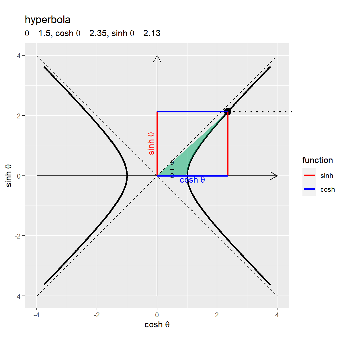
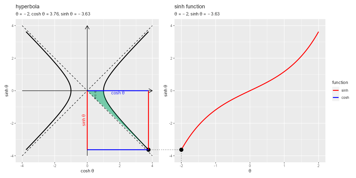
最後は、双曲線上におけるsinh関数の値(直線)と、sinh関数の曲線の関係をグラフで確認します。
グラフの作成
変数を固定したグラフで確認します。
・作図コード(クリックで展開)
双曲線上の点とsinh曲線上の点を結ぶ補助線(の半分)を描画するためのデータフレームを作成します。
# sinh曲線との対応用
l <- 0.5
segment_hyperbola_df <- tibble::tibble(
  x_from = cosh(theta),
  x_to = axis_max+l,
  y = sinh(theta)
)
segment_hyperbola_df
## # A tibble: 1 × 3
##   x_from  x_to     y
##    <dbl> <dbl> <dbl>
## 1   2.35   4.5  2.13
曲線上の点からy軸の反対側への垂線を引くように座標を指定します。
双曲線のグラフを作成します。
# 変数ラベルの描画用
hyperbola_label <- paste0(
  "list(",
  "theta==", theta,
  ", cosh~theta==", round(cosh(theta), digits = 2),
  ", sinh~theta==", round(sinh(theta), digits = 2),
  ")"
)

# 双曲線関数を作図
hyperbola_graph <- ggplot() +
  geom_segment(data = axis_df,
               mapping = aes(x = x_from, y = y_from, xend = x_to, yend = y_to, group = "axis"),
               arrow = arrow(length = unit(10, units = "pt"))) + # 軸線
  geom_line(data = asymptote_df,
            mapping = aes(x = x, y = y, group = slope),
            linetype = "dashed") + # 漸近線
  geom_path(data = hyperbola_df,
            mapping = aes(x = cosh_t, y = sinh_t, group = sign),
            size = 1) + # 双曲線
  geom_point(data = point_df,
             mapping = aes(x = cosh_t, y = sinh_t),
             size = 4) + # 双曲線上の点
  geom_ribbon(data = variable_area_df,
              mapping = aes(x = x, ymin = curve, ymax = straight),
              fill = "#00A968", alpha = 0.5) + # 変数(面積)
  geom_text(mapping = aes(x = 0.5, y = 0.25*tanh(theta), label = "frac(theta, 2)"), parse = TRUE,
            size = 3) + # 変数ラベル
  geom_segment(data = segment_hyperbola_df,
               mapping = aes(x = x_from, y = y, xend = x_to, yend = y),
               size = 1, linetype = "dotted") + # sinh曲線との対応線
  geom_segment(data = function_df,
               mapping = aes(x = x_from, y = y_from, xend = x_to, yend = y_to, color = fnc),
               size = 1) + # 双曲線関数直線
  geom_text(data = function_label_df,
            mapping = aes(x = x, y = y, label = fnc_label, color = fnc, angle = angle, vjust = v), parse = TRUE,
            show.legend = FALSE) + # 双曲線関数ラベル
  scale_color_manual(breaks = c("sinh", "cosh"),
                     values = c("red", "blue")) +
  coord_fixed(ratio = 1, clip = "off",
              xlim = c(-axis_max, axis_max), ylim = c(-axis_max, axis_max)) + # 表示範囲
  labs(title = "hyperbola",
       subtitle = parse(text = hyperbola_label),
       color = "function",
       x = expression(cosh~theta), y = expression(sinh~theta))
hyperbola_graph
sinh曲線上の点と双曲線上の点を結ぶ補助線(の半分)を描画するためのデータフレームを作成します。
# 双曲線との対応用
d <- 1.1
l <- 0.6
segment_sinh_df <- tibble::tibble(
  x_from = c(theta, theta),
  y_from = c(sinh(theta), sinh(theta)),
  x_to = c(theta, min(theta_vec)-l),
  y_to = c(-axis_max*d, sinh(theta))
)
segment_sinh_df
## # A tibble: 2 × 4
##   x_from y_from  x_to  y_to
##    <dbl>  <dbl> <dbl> <dbl>
## 1    1.5   2.13   1.5 -4.4
## 2    1.5   2.13  -2.6  2.13
曲線上の点からx軸とy軸への垂線を引くように座標を指定します。
sinh関数曲線のグラフを作成します。
# sinh曲線の描画用
sinh_df <- tibble::tibble(
  t = theta_vec,
  sinh_t = sinh(theta_vec)
)

# 関数ラベルの描画用
sinh_label <- paste0(
  "list(",
  "theta==", theta,
  ", sinh~theta==", round(sinh(theta), digits = 2),
  ")"
)

# sinh関数を作図
sinh_graph <- ggplot() +
  geom_line(data = sinh_df,
            mapping = aes(x = t, y = sinh_t),
            color = "red", size = 1) + # sinh曲線
  geom_segment(data = segment_sinh_df,
               mapping = aes(x = x_from, y = y_from, xend = x_to, yend = y_to),
               size = 1, linetype = "dotted") + # 双曲線との対応線
  geom_point(data = point_df,
             mapping = aes(x = t, y = sinh_t),
             size = 4) + #sinh曲線上の点
  coord_cartesian(clip = "off",
                  xlim = c(min(theta_vec), max(theta_vec)), ylim = c(-axis_max, axis_max)) + #
  labs(title = "sinh function",
       subtitle = parse(text = sinh_label),
       x = expression(theta), y = expression(sinh~theta))
sinh_graph
2つのグラフを並べて描画します。
# 並べて描画
patchwork::wrap_plots(hyperbola_graph, sinh_graph, guides = "collect")
patchworkパッケージのwrap_plots()を使ってグラフを並べます。
双曲線のグラフにおける高さがsinh関数の曲線に対応しているのを確認できます。
アニメーションの作成
続いて、変数の値を変化させたアニメーションで確認します。
フレーム数を指定して、変数として用いる値を作成します。
# フレーム数を指定
frame_num <- 101

# 変数の値を作成
theta_i <- seq(from = -2, to = 2, length.out = frame_num) # 範囲を指定
head(theta_i)
## [1] -2.00 -1.96 -1.92 -1.88 -1.84 -1.80
フレーム数frame_numを指定して、frame_num個の$\theta$の値を作成します。
・作図コード(クリックで展開)
theta_iから順番に値を取り出して作図し、グラフを書き出します。
# 一時保存フォルダを指定
dir_path <- "tmp_folder"

# 関数ラベルのレベルを指定
fnc_level_vec <- c("sinh", "cosh")

# 変数ごとに作図
for(i in 1:frame_num) {

  # i番目の値を取得
  theta <- theta_i[i]

  # 曲線上の点の描画用
  point_df <- tibble::tibble(
    t = theta,
    sinh_t = sinh(theta),
    cosh_t = cosh(theta)
  )

  # 変数(面積)の描画用
  variable_area_df <- tibble::tibble(
    x = seq(from = 0, to = cosh(theta), length.out = 50),
    sign = dplyr::if_else(theta >= 0, true = 1, false = -1), # 符号
    curve = sign * sqrt(x^2 - 1), # x軸と双曲線上の線分
    straight = sinh(theta)/cosh(theta) * x # 原点と曲線上の点の線分
  ) |>
    dplyr::mutate(
      curve = dplyr::if_else(is.na(curve), true = 0, false = curve)
    ) # 双曲線の範囲外を0に置換

  # 双曲線関数の描画用
  function_df <- tibble::tibble(
    x_from = c(0, cosh(theta), 0, 0),
    y_from = c(0, 0, 0, sinh(theta)),
    x_to = c(0, cosh(theta), cosh(theta), cosh(theta)),
    y_to = c(sinh(theta), sinh(theta), 0, sinh(theta)),
    fnc = c("sinh", "sinh", "cosh", "cosh") |>
      factor(levels = fnc_level_vec) # 色分け用
  )

  # 双曲線関数ラベルの描画用
  function_label_df <- tibble::tibble(
    x = c(0, 0.5*cosh(theta)),
    y = c(0.5*sinh(theta), 0),
    angle = c(90, 0),
    v = c(-0.5, 1),
    fnc = c("sinh", "cosh") |>
      factor(levels = fnc_level_vec), # 色分け用
    fnc_label = c("sinh~theta", "cosh~theta") # 関数ラベル
  )

  # sinh曲線との対応用
  l <- 0.5
  segment_hyperbola_df <- tibble::tibble(
    x_from = cosh(theta),
    x_to = axis_max+l,
    y = sinh(theta)
  )

  # 変数ラベルの描画用
  hyperbola_label <- paste0(
    "list(",
    "theta==", theta,
    ", cosh~theta==", round(cosh(theta), digits = 2),
    ", sinh~theta==", round(sinh(theta), digits = 2),
    ")"
  )

  # 双曲線関数を作図
  hyperbola_graph <- ggplot() +
    geom_segment(data = axis_df,
                 mapping = aes(x = x_from, y = y_from, xend = x_to, yend = y_to, group = "axis"),
                 arrow = arrow(length = unit(10, units = "pt"))) + # 軸線
    geom_line(data = asymptote_df,
              mapping = aes(x = x, y = y, group = slope),
              linetype = "dashed") + # 漸近線
    geom_path(data = hyperbola_df,
              mapping = aes(x = cosh_t, y = sinh_t, group = sign),
              size = 1) + # 双曲線
    geom_point(data = point_df,
               mapping = aes(x = cosh_t, y = sinh_t),
               size = 4) + # 双曲線上の点
    geom_ribbon(data = variable_area_df,
                mapping = aes(x = x, ymin = curve, ymax = straight),
                fill = "#00A968", alpha = 0.5) + # 変数(面積)
    geom_text(mapping = aes(x = 0.5, y = 0.25*tanh(theta), label = "frac(theta, 2)"), parse = TRUE,
              size = 3) + # 変数ラベル
    geom_segment(data = segment_hyperbola_df,
                 mapping = aes(x = x_from, y = y, xend = x_to, yend = y),
                 linetype = "dotted") + # sinh曲線との対応線
    geom_segment(data = function_df,
                 mapping = aes(x = x_from, y = y_from, xend = x_to, yend = y_to, color = fnc),
                 size = 1) + # 双曲線関数直線
    geom_text(data = function_label_df,
              mapping = aes(x = x, y = y, label = fnc_label, color = fnc, angle = angle, vjust = v), parse = TRUE,
              show.legend = FALSE) + # 双曲線関数ラベル
    scale_color_manual(breaks = c("sinh", "cosh"),
                       values = c("red", "blue")) +
    coord_fixed(ratio = 1, clip = "off",
                xlim = c(-axis_max, axis_max), ylim = c(-axis_max, axis_max)) + # 表示範囲
    labs(title = "hyperbola",
         subtitle = parse(text = hyperbola_label),
         color = "function",
         x = expression(cosh~theta), y = expression(sinh~theta))

  # sinh曲線の描画用
  sinh_df <- tibble::tibble(
    t = theta_vec,
    sinh_t = sinh(theta_vec)
  )

  # 双曲線との対応用
  d <- 1.1
  l <- 0.6
  segment_sinh_df <- tibble::tibble(
    x_from = c(theta, theta),
    y_from = c(sinh(theta), sinh(theta)),
    x_to = c(theta, min(theta_vec)-l),
    y_to = c(-axis_max*d, sinh(theta))
  )

  # 関数ラベルの描画用
  sinh_label <- paste0(
    "list(",
    "theta==", theta,
    ", sinh~theta==", round(sinh(theta), digits = 2),
    ")"
  )

  # sinh関数を作図
  sinh_graph <- ggplot() +
    geom_line(data = sinh_df,
              mapping = aes(x = t, y = sinh_t),
              color = "red", size = 1) + # sinh曲線
    geom_segment(data = segment_sinh_df,
                 mapping = aes(x = x_from, y = y_from, xend = x_to, yend = y_to),
                 linetype = "dotted") + # 双曲線との対応線
    geom_point(data = point_df,
               mapping = aes(x = t, y = sinh_t),
               size = 4) + #sinh曲線上の点
    coord_cartesian(clip = "off",
                    xlim = c(min(theta_vec), max(theta_vec)), ylim = c(-axis_max, axis_max)) + #
    labs(title = "sinh function",
         subtitle = parse(text = sinh_label),
         x = expression(theta), y = expression(sinh~theta))

  # 並べて描画
  graph <- patchwork::wrap_plots(hyperbola_graph, sinh_graph, guides = "collect")

  # ファイルを書き出し
  file_path <- paste0(dir_path, "/", stringr::str_pad(i, width = nchar(frame_num), pad = "0"), ".png")
  ggplot2::ggsave(filename = file_path, plot = graph, width = 1200, height = 600, units = "px", dpi = 100)

  # 途中経過を表示
  message("\r", i, " / ", frame_num, appendLF = FALSE)
}
変数の値ごとに「グラフの作成」と同様に処理します。作成したグラフをggsave()で保存します。
sinh関数のアニメーションを作成します。
# gif画像を作成
paste0(dir_path, "/", stringr::str_pad(1:frame_num, width = nchar(frame_num), pad = "0"), ".png") |> # ファイルパスを作成
  magick::image_read() |> # 画像ファイルを読込
  magick::image_animate(fps = 1, dispose = "previous") |> # gif画像を作成
  magick::image_write_gif(path = "sinh.gif", delay = 0.1) -> tmp_path # gifファイル書き出
全てのファイルパスを作成して、image_read()で画像ファイルを読み込んで、image_animate()でgif画像に変換して、image_write_gif()でgifファイルを書き出します。delay引数に1秒当たりのフレーム数の逆数を指定します。
双曲線上の点の高さに応じて推移するのを確認できます。
この記事では、sinh関数を可視化しました。次の記事では、cosh関数を可視化します。
おわりに
tanh関数に続いて双曲線関数シリーズ2つ目の記事ですが、シリーズ的にはこっちを1つ目とした方が流れがいいですね。残り4つもやるつもりです。
2023年2月22日は、モーニング娘。'23の横山玲奈さんの22歳のお誕生日です。(サムネの左上の方です)
よこにゃーん🐨
【次の内容】