はじめに
R言語で三角関数の定義や公式を可視化しようシリーズです。
この記事では、2つの角の差に関する三角関数の加法定理のグラフを作成します。
【前の内容】
【他の記事一覧】
【この記事の内容】
三角関数の加法定の可視化理:その2(2角の差)
三角関数における加法定理(2つの角の差のサインとコサイン)を可視化します。
利用するパッケージを読み込みます。
# 利用パッケージ
library(tidyverse)
library(gganimate)
この記事では、基本的にパッケージ名::関数名()の記法を使うので、パッケージを読み込む必要はありません。ただし、作図コードがごちゃごちゃしないようにパッケージ名を省略しているためggplot2を読み込む必要があります。
また、ネイティブパイプ演算子|>を使っています。magrittrパッケージのパイプ演算子%>%に置き換えても処理できますが、その場合はmagrittrも読み込む必要があります。
加法定理の公式
三角関数の加法定理として、次の関係が成り立ちます。
この記事では、$\sin(\alpha - \beta)$と$\cos(\alpha - \beta)$の式に関して可視化して確認します。
加法定理の可視化
三角関数の加法定理($\sin(\alpha - \beta), \cos(\alpha - \beta)$)をグラフで確認します。
グラフの作成
まずは、角度を固定したグラフを作成します。
角度を指定して、ラジアンに変換します。
# 角度を指定
a <- 60
b <- 15

# ラジアンに変換
alpha <- a / 180 * pi
beta  <- b / 180 * pi
alpha; beta
## [1] 1.047198
## [1] 0.2617994
度数法における角度$0^{\circ} \leq a \leq 90^{\circ}$、$0^{\circ} \leq b \leq a$を指定します。
指定した角度を、弧度法におけるラジアン$\alpha = a \frac{2 \pi}{360}$、$\beta = b \frac{2 \pi}{360}$に変換します。$\pi$は円周率でpiで扱えます。
・コード(クリックで展開)
(第1象限における)単位円を描画するためのデータフレームを作成します。
# 単位円(の4分の1)の描画用
sector_df <- tibble::tibble(
  c = seq(from = 0, to = 90, by = 1),
  theta = c / 180 * pi,
  x = cos(theta),
  y = sin(theta)
)
sector_df
## # A tibble: 91 × 4
##        c  theta     x      y
##    <dbl>  <dbl> <dbl>  <dbl>
##  1     0 0      1     0
##  2     1 0.0175 1.00  0.0175
##  3     2 0.0349 0.999 0.0349
##  4     3 0.0524 0.999 0.0523
##  5     4 0.0698 0.998 0.0698
##  6     5 0.0873 0.996 0.0872
##  7     6 0.105  0.995 0.105
##  8     7 0.122  0.993 0.122
##  9     8 0.140  0.990 0.139
## 10     9 0.157  0.988 0.156
## # … with 81 more rows
作図用の角度$0^{\circ} \leq c \leq 90^{\circ}$を作成して、ラジアン$\theta = c \frac{2 \pi}{360}$に変換します。
x軸の値は$x = \cos \theta$、y軸の値は$y = \sin \theta$で単位円を描くための点の座標を計算します。
単位正方形を描画するためのデータフレームを作成します。
# 単位正方形の描画用
square_df <- tibble::tibble(
  x = c(0, 0, 1, 1, 0),
  y = c(0, 1, 1, 0, 0)
)
square_df
## # A tibble: 5 × 2
##       x     y
##   <dbl> <dbl>
## 1     0     0
## 2     0     1
## 3     1     1
## 4     1     0
## 5     0     0
単位正方形の頂点の座標を格納します。
加法定理を構成する辺(線分)を描画するためのデータフレームを作成します。
# 因子レベルを指定
fnc_level <- c(
  "r", "sin(a)", "cos(a)",
  "sin(a) sin(b)", "cos(a) sin(b)",
  "sub1", "sub2",
  "cos(a) cos(b)", "sin(a) cos(b)",
  "sin(a-b)", "cos(a-b)"
)

# 辺の描画用
A_x <- cos(alpha)*cos(beta)^2
A_y <- cos(alpha)*sin(beta)*cos(beta)
B_x <- cos(alpha)-sin(alpha)*sin(beta)*cos(beta)
B_y <- sin(alpha)-sin(alpha)*sin(beta)^2
C_x <- cos(alpha)+sin(alpha)*sin(beta)*cos(beta)
C_y <- sin(alpha)*sin(beta)^2
segment_df <- tibble::tribble(
  ~fnc,            ~type,    ~label, ~width,   ~x_from, ~y_from,       ~x_to,                     ~y_to,
  "r",             "main",   TRUE,   "normal", 0,          0,             cos(alpha),                sin(alpha),
  "sin(a)",        "main",   TRUE,   "normal", cos(alpha), sin(alpha),    cos(alpha),                0,
  "cos(a)",        "main",   TRUE,   "normal", 0,          0,             cos(alpha),                0,
  "cos(a) cos(b)", "main",   TRUE,   "normal", 0,          0,             A_x,                       A_y,
  "sin(a) sin(b)", "main",   TRUE,   "normal", cos(alpha), sin(alpha),    B_x,                       B_y,
  "sin(a) sin(b)", "main",   FALSE,  "normal", A_x,        A_y,           cos(alpha-beta)*cos(beta), cos(alpha-beta)*sin(beta),
  "sin(a) sin(b)", "main",   FALSE,  "normal", cos(alpha), 0,             C_x,                       C_y,
  "sin(a) cos(b)", "main",   TRUE,   "normal", cos(alpha), 0,             B_x,                       B_y,
  "sin(a) cos(b)", "main",   FALSE,  "normal", cos(alpha), sin(alpha),    C_x,                       C_y,
  "cos(a) sin(b)", "main",   FALSE,  "bold",   cos(alpha), 0,             A_x,                       A_y,
  "cos(a) sin(b)", "main",   TRUE,   "bold",   C_x,        C_y,           cos(alpha-beta)*cos(beta), cos(alpha-beta)*sin(beta),
  "sin(a-b)",      "target", TRUE,   "bold",   cos(alpha), sin(alpha),    cos(alpha-beta)*cos(beta), cos(alpha-beta)*sin(beta),
  "cos(a-b)",      "target", TRUE,   "bold",   0,          0,             cos(alpha-beta)*cos(beta), cos(alpha-beta)*sin(beta),
  "r",             "sub",    FALSE,  "normal", cos(beta),  sin(beta),     cos(alpha-beta)*cos(beta), cos(alpha-beta)*sin(beta),
  "sub1",          "sub",    FALSE,  "normal", cos(alpha), 0,             C_x,                       0,
  "sub1",          "sub",    FALSE,  "normal", cos(alpha), sin(alpha),    B_x,                       sin(alpha),
  "sub2",          "sub",    FALSE,  "normal", C_x,        0,             C_x,                       C_y,
  "sub2",          "sub",    FALSE,  "normal", B_x,        sin(alpha),    B_x,                       B_y
  ) |> # 座標を格納
  dplyr::mutate(
    fnc = factor(fnc, levels = fnc_level) # 因子レベルを設定
  ) |>
  dplyr::arrange(fnc) # 並びを統一
segment_df
## # A tibble: 18 × 8
##    fnc           type   label width  x_from y_from  x_to   y_to
##    <fct>         <chr>  <lgl> <chr>   <dbl>  <dbl> <dbl>  <dbl>
##  1 r             main   TRUE  normal  0     0      0.5   0.866
##  2 r             sub    FALSE normal  0.966 0.259  0.683 0.183
##  3 sin(a)        main   TRUE  normal  0.5   0.866  0.5   0
##  4 cos(a)        main   TRUE  normal  0     0      0.5   0
##  5 sin(a) sin(b) main   TRUE  normal  0.5   0.866  0.283 0.808
##  6 sin(a) sin(b) main   FALSE normal  0.467 0.125  0.683 0.183
##  7 sin(a) sin(b) main   FALSE normal  0.5   0      0.717 0.0580
##  8 cos(a) sin(b) main   FALSE bold    0.5   0      0.467 0.125
##  9 cos(a) sin(b) main   TRUE  bold    0.717 0.0580 0.683 0.183
## 10 sub1          sub    FALSE normal  0.5   0      0.717 0
## 11 sub1          sub    FALSE normal  0.5   0.866  0.283 0.866
## 12 sub2          sub    FALSE normal  0.717 0      0.717 0.0580
## 13 sub2          sub    FALSE normal  0.283 0.866  0.283 0.808
## 14 cos(a) cos(b) main   TRUE  normal  0     0      0.467 0.125
## 15 sin(a) cos(b) main   TRUE  normal  0.5   0      0.283 0.808
## 16 sin(a) cos(b) main   FALSE normal  0.5   0.866  0.717 0.0580
## 17 sin(a-b)      target TRUE  bold    0.5   0.866  0.683 0.183
## 18 cos(a-b)      target TRUE  bold    0     0      0.683 0.183
各辺の値を格納しやすいように、tribble()を使ってデータフレームを作成します。線分の始点の座標をx_from, y_from列、終点の座標をx_to, y_to列とします。次の「関数名ラベル」の関数の値は線分の長さであり、座標の値とは異なります。
各関数(辺)を区別するためのfnc列、「加法定理を示す線("target)」・「加法定理を求めるための線("main)」・「補助線("sub)」を区別するためのtype列を作成します。fnc列は色分け、type列は線の種類に使います。
平行な同じ長さの辺はfnc列を同じ値とします。ただし、関数名ラベルは1辺のみに描画することにします。ラベルの有無をlabel列で設定します。ラベルを付ける辺はTRUE、付けない辺はFALSEにします。
線が重なる辺があるので、width列で線の太さを設定します。通常を"normal"とし、重なる線(の片方)を"bold"とします。
線の描画順(重なり順)や色付け順は、fnc列の因子レベルに依存するので、fnc_levelとして指定しておきます。
線分ごとに関数名ラベルを描画するためのデータフレームを作成します。
# 関数名ラベルの描画用
segment_label_df <- segment_df |>
  dplyr::filter(label) |>
  dplyr::group_by(fnc) |> # 中点の計算用
  dplyr::mutate(
    # 線分の中点に配置
    x = median(c(x_from, x_to)),
    y = median(c(y_from, y_to))
  ) |>
  dplyr::ungroup() |>
  tibble::add_column(
    # ラベルが重ならないように調整
    h = c(1.0, 0.5, 0.5, 0.5, 0.0, 0.5, 0.5, 0.0, 0.5),
    v = c(0.5, 0.5, 1.0, 0.0, 0.5, 1.0, 0.5, 0.5, 0.0),
    # ラベルを作成
    fnc_label = c(
      "r==1",
      paste0("sin~alpha==", round(sin(alpha), digits = 2)),
      paste0("cos~alpha==", round(cos(alpha), digits = 2)),
      paste0("sin~alpha ~ sin~beta==", round(sin(alpha)*sin(beta), digits = 2)),
      paste0("cos~alpha ~ sin~beta==", round(cos(alpha)*sin(beta), digits = 2)),
      paste0("cos~alpha ~ cos~beta==", round(cos(alpha)*cos(beta), digits = 2)),
      paste0("sin~alpha ~ cos~beta==", round(sin(alpha)*cos(beta), digits = 2)),
      paste0("sin(alpha-beta)==", round(sin(alpha-beta), digits = 2)),
      paste0("cos(alpha-beta)==", round(cos(alpha-beta), digits = 2))
    )
  ) |>
  dplyr::select(fnc, fnc_label, x, y, h, v)
segment_label_df
## # A tibble: 9 × 6
##   fnc           fnc_label                      x      y     h     v
##   <fct>         <chr>                      <dbl>  <dbl> <dbl> <dbl>
## 1 r             r==1                       0.25  0.433    1     0.5
## 2 sin(a)        sin~alpha==0.87            0.5   0.433    0.5   0.5
## 3 cos(a)        cos~alpha==0.5             0.25  0        0.5   1
## 4 sin(a) sin(b) sin~alpha ~ sin~beta==0.22 0.392 0.837    0.5   0
## 5 cos(a) sin(b) cos~alpha ~ sin~beta==0.13 0.700 0.121    0     0.5
## 6 cos(a) cos(b) cos~alpha ~ cos~beta==0.48 0.233 0.0625   0.5   1
## 7 sin(a) cos(b) sin~alpha ~ cos~beta==0.84 0.392 0.404    0.5   0.5
## 8 sin(a-b)      sin(alpha-beta)==0.71      0.592 0.525    0     0.5
## 9 cos(a-b)      cos(alpha-beta)==0.71      0.342 0.0915   0.5   0
ラベル付けする辺(label列がTRUEの行)を取り出して、各線分の中点にラベルを配置することにします。
辺ごとに(fnc列でグループ化して)、x軸の値はx_from, x_to列、y軸の値はy_from, y_to列の中央値を計算します。
ラベルとして数式を表示するにはexpression()の記法を使います。
直角を示すためのデータフレームを作成します。
# 直角マークの描画用
d <- 0.03
right_angle_df <- tibble::tibble(
  x = c(
    cos(alpha) + c(0, -d, -d),
    C_x + c(0, -d, -d),
    C_x + c(cos(beta+0.5*pi)*d, cos(beta+0.5*pi)*d+cos(beta+pi)*d, cos(beta+pi)*d),
    cos(alpha-beta)*cos(beta) + c(cos(beta+0.5*pi)*d, cos(beta+0.5*pi)*d+cos(beta+pi)*d, cos(beta+pi)*d),
    B_x + c(d, d, 0),
    B_x + c(cos(beta)*d, cos(beta)*d+cos(beta+1.5*pi)*d, cos(beta+1.5*pi)*d)
  ),
  y = c(
    0 + c(d, d, 0),
    0 + c(d, d, 0),
    C_y + c(sin(beta+0.5*pi)*d, sin(beta+0.5*pi)*d+sin(beta+pi)*d, sin(beta+pi)*d),
    cos(alpha-beta)*sin(beta) + c(sin(beta+0.5*pi)*d, sin(beta+0.5*pi)*d+sin(beta+pi)*d, sin(beta+pi)*d),
    sin(alpha) + c(0, -d, -d),
    B_y + c(sin(beta)*d, sin(beta)*d+sin(beta+1.5*pi)*d, sin(beta+1.5*pi)*d)
  ),
  id = rep(1:6, each = 3) # 角ラベル
)
right_angle_df
## # A tibble: 18 × 3
##        x      y    id
##    <dbl>  <dbl> <int>
##  1 0.5   0.03       1
##  2 0.47  0.03       1
##  3 0.47  0          1
##  4 0.717 0.03       2
##  5 0.687 0.03       2
##  6 0.687 0          2
##  7 0.709 0.0870     3
##  8 0.680 0.0792     3
##  9 0.688 0.0502     3
## 10 0.675 0.212      4
## 11 0.646 0.204      4
## 12 0.654 0.175      4
## 13 0.313 0.866      5
## 14 0.313 0.836      5
## 15 0.283 0.836      5
## 16 0.312 0.816      6
## 17 0.320 0.787      6
## 18 0.291 0.779      6
直角マークの頂点の座標を計算して格納します。
鋭角を示すためのデータフレームを作成します。
# 因子レベルを指定
ang_level <- c("a", "b", "90-b", "a-b")

# 角度マーク(扇形)の描画用
angle_df <- dplyr::bind_rows(
  # 原点を中心とする角度
  tibble::tibble(
    ang = c(
      rep("a", times = a+1),
      rep("b", times = b+1),
      rep("90-b", times = 90-b+1),
      rep("a-b", times = a-b+1)
    ) |>
      factor(levels = ang_level), # 角ラベル
    id = dplyr::dense_rank(ang), # 角番号
    x0 = 0,
    y0 = 0,
    c = c(
      seq(from = 0, to = a, by = 1),
      seq(from = 0, to = b, by = 1),
      seq(from = b, to = 90, by = 1),
      seq(from = b, to = a, by = 1)
    ) # 角度
  ),
  # 点(cos α, 0)を中心とする角度
  tibble::tibble(
    ang = c(
      rep("b", times = b+1),
      rep("90-b", times = 90-b+1),
      rep("b", times = b+1),
      rep("90-b", times = 90-b+1)
    ) |>
      factor(levels = ang_level), # 角ラベル
    id = c(
      rep(5, times = b+1),
      rep(6, times = 90-b+1),
      rep(7, times = b+1),
      rep(8, times = 90-b+1)
    ), # 角番号
    x0 = cos(alpha),
    y0 = 0,
    c = c(
      seq(from = 0, to = b, by = 1),
      seq(from = b, to = 90, by = 1),
      seq(from = 90, to = 90+b, by = 1),
      seq(from = 90+b, to = 180, by = 1)
    ) # 角度
  ),
  # 点(cos α, sin β)を中心とする角度
  tibble::tibble(
    ang = c(
      rep("b", times = b+1),
      rep("90-b", times = 90-b+1),
      rep("b", times = b+1)
    ) |>
      factor(levels = ang_level), # 角ラベル
    id = c(
      rep(9, times = b+1),
      rep(10, times = 90-b+1),
      rep(11, times = b+1)
    ), # 角番号
    x0 = cos(alpha),
    y0 = sin(alpha),
    c = c(
      seq(from = 180, to = 180+b, by = 1),
      seq(from = 180+b, to = 270, by = 1),
      seq(from = 270, to = 270+b, by = 1)
    ) # 角度
  )
) |>
  dplyr::mutate(
    theta = c / 180 * pi, # ラジアン
    d = dplyr::case_when(
      ang == "a" ~ 0.05,
      ang == "b" ~ 0.06,
      ang == "90-b" ~ 0.06,
      ang == "a-b" ~ 0.07
    ), # サイズ調整用の値を指定
    # 角ごとに配置
    x = cos(theta) * d + x0,
    y = sin(theta) * d + y0
 )
angle_df
## # A tibble: 491 × 9
##    ang      id    x0    y0     c  theta     d      x        y
##    <fct> <dbl> <dbl> <dbl> <dbl>  <dbl> <dbl>  <dbl>    <dbl>
##  1 a         1     0     0     0 0       0.05 0.05   0
##  2 a         1     0     0     1 0.0175  0.05 0.0500 0.000873
##  3 a         1     0     0     2 0.0349  0.05 0.0500 0.00174
##  4 a         1     0     0     3 0.0524  0.05 0.0499 0.00262
##  5 a         1     0     0     4 0.0698  0.05 0.0499 0.00349
##  6 a         1     0     0     5 0.0873  0.05 0.0498 0.00436
##  7 a         1     0     0     6 0.105   0.05 0.0497 0.00523
##  8 a         1     0     0     7 0.122   0.05 0.0496 0.00609
##  9 a         1     0     0     8 0.140   0.05 0.0495 0.00696
## 10 a         1     0     0     9 0.157   0.05 0.0494 0.00782
## # … with 481 more rows
3つの頂点において複数の角度マークを描画します。
扇形(角度マーク)を描画するための点の角度($0^{\circ} \leq c \leq a$など)を作成して、それぞれラジアン$\theta = c \frac{2 \pi}{360}$に変換して、$x = \cos \theta, y = \sin \theta$で原点を頂点(円の中心)としたときの座標に変換し、角ごとに頂点の座標$x_0, y_0$を加えてプロット位置を変更します。
角を区別するための列(同じ角度の角は同じ文字列)ang、角番号列(角ごとのユニークな通し番号)id、頂点の座標列x0, y0、扇形描画用の点の角度列cを、頂点ごとにデータフレームに格納して、bind_rows()で結合します。全ての頂点のデータを結合した後に、座標を計算します。
扇形のサイズ調整用の値をd列として、角度ごとに値を指定します。
角度ラベルを描画するためのデータフレームを作成します。
# 角度ラベルの描画用
angle_label_df <- angle_df |>
  dplyr::group_by(id, ang, x0, y0) |> # 中点の計算用
  dplyr::summarise(
    # 角度の中点に配置
    c = median(c), .groups = "drop"
  ) |>
  dplyr::mutate(
    theta = c / 180 * pi, # ラジアン
    angle_label = dplyr::case_when(
      ang == "a" ~ "alpha",
      ang == "b" ~ "beta",
      ang == "90-b" ~ "90*degree-beta",
      ang == "a-b" ~ "alpha-beta"
    ), # 角度ラベル
    d = dplyr::case_when(
      ang == "a" ~ 0.04,
      ang == "b" ~ 0.09,
      ang == "90-b" ~ 0.1,
      ang == "a-b" ~ 0.1
    ), # サイズ調整用の値を指定
    # 角ごとに配置
    x = cos(theta) * d + x0,
    y = sin(theta) * d + y0
  )
angle_label_df
## # A tibble: 11 × 10
##       id ang      x0    y0     c theta angle_label        d      x      y
##    <dbl> <fct> <dbl> <dbl> <dbl> <dbl> <chr>          <dbl>  <dbl>  <dbl>
##  1     1 a       0   0      30   0.524 alpha           0.04 0.0346 0.02
##  2     2 b       0   0       7.5 0.131 beta            0.09 0.0892 0.0117
##  3     3 90-b    0   0      52.5 0.916 90*degree-beta  0.1  0.0609 0.0793
##  4     4 a-b     0   0      37.5 0.654 alpha-beta      0.1  0.0793 0.0609
##  5     5 b       0.5 0       7.5 0.131 beta            0.09 0.589  0.0117
##  6     6 90-b    0.5 0      52.5 0.916 90*degree-beta  0.1  0.561  0.0793
##  7     7 b       0.5 0      97.5 1.70  beta            0.09 0.488  0.0892
##  8     8 90-b    0.5 0     142.  2.49  90*degree-beta  0.1  0.421  0.0609
##  9     9 b       0.5 0.866 188.  3.27  beta            0.09 0.411  0.854
## 10    10 90-b    0.5 0.866 232.  4.06  90*degree-beta  0.1  0.439  0.787
## 11    11 b       0.5 0.866 278.  4.84  beta            0.09 0.512  0.777
角ごとに角度の中点に配置することにします。
角ごとに(ang列と中央値の計算後に利用する列でグループ化して)、summarise()を使って角度の中央値を計算して、それぞれ座標を計算します。
加法定理の可視化グラフを作成します。
# タイトル用のラベルを作成
title_label <- paste0(
  "atop(",
  "sin~(alpha-beta) == sin~alpha ~ cos~beta - cos~alpha ~ sin~beta",
  ", cos~(alpha-beta) == cos~alpha ~ cos~beta + sin~alpha ~ sin~beta",
  ")"
)
ver_label <- paste0(
  "list(",
  "a==", a, "*degree", ", b==", b, "*degree",
  ", alpha==", round(a/180, 2), "*pi, beta==", round(b/180, 2), "*pi",
  ")"
)

# 加法定理の可視化
ggplot() +
  geom_path(data = sector_df,
            mapping = aes(x = x, y = y),
            size = 1) + # 単位円
  geom_path(data = square_df,
            mapping = aes(x = x, y = y),
            linetype = "dotted") + # 単位正方形
  geom_segment(data = segment_df,
               mapping = aes(x = x_from, y = y_from, xend = x_to, yend = y_to,
                             color = fnc, size = width, linetype = type)) + # 関数の線分
  geom_path(data = right_angle_df,
            mapping = aes(x = x, y = y, group = id)) + # 直角マーク
  geom_path(data = angle_df,
            mapping = aes(x = x, y = y, linetype = ang, group = id)) + # 角度マーク
  geom_text(data = angle_label_df,
            mapping = aes(x = x, y = y, label = angle_label), parse = TRUE) + # 角度ラベル
  geom_label(data = segment_label_df,
             mapping = aes(x = x, y = y, label = fnc_label, hjust = h, vjust = v, color = fnc), parse = TRUE,
             alpha = 0.5) + # 関数名ラベル
  scale_size_manual(breaks = c("normal", "bold"),
                    values = c(1, 2)) + #  目的の線を強調
  scale_linetype_manual(breaks = c("main", "sub", "target", "a", "b", "90-b", "a-b"),
                        values = c("solid", "dotted", "dashed", "solid", "solid", "dashed", "solid")) + #  目的の線を強調
  #scale_color_brewer(palette = "Set1") +
  theme(legend.position = "none") + # 凡例を非表示
  coord_fixed(ratio = 1, clip = "off") + # アスペクト比
  labs(title = parse(text = title_label),
       subtitle = parse(text = ver_label),
       x = "x", y = "y")
単位円(扇形の線)をgeom_path()、線分をgeom_segment()、ラベル(文字列)をgeom_text()またはgeom_label()で描画します。ラベルとして数式を描画する場合は、parse引数をTRUEにします。
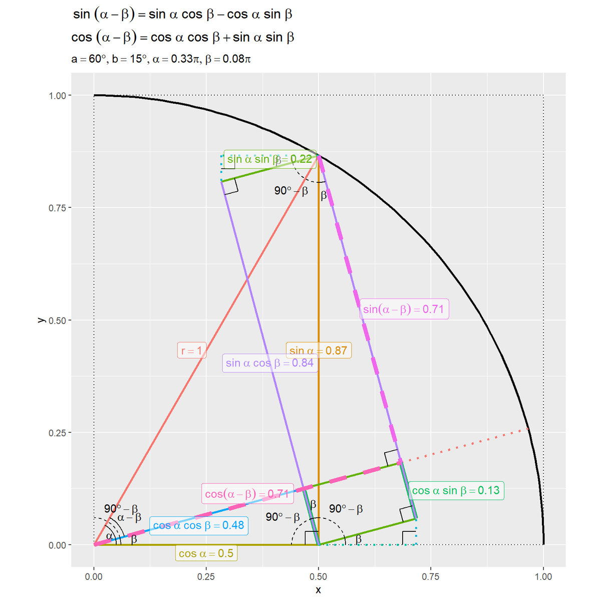
2つの破線とそれぞれ平行な実線を比較すると、次の関係が成り立つのが分かります。
$\sin \alpha \cos \beta$の辺(紫色の線分)は、$\cos \alpha \sin \beta$の辺(青緑色の線分)の全体と重なっています。
アニメーションの作成
次は、角度と加法定理の関係をアニメーションで確認します。
フレームごとに変化させる角度を指定して、ラジアンに変換します。
# フレーム数を指定
frame_num <- 61

# 角度として利用する値を指定:(a,αを変化させる場合)
a_vals <- seq(from = 30, to = 90, length.out = frame_num)
b_vals <- rep(30, times = frame_num)

# 角度として利用する値を指定:(b,βを変化させる場合)
#a_vals <- rep(60, times = frame_num)
#b_vals <- seq(from = 0, to = 60, length.out = frame_num)

# ラジアンに変換
alpha_vals <- a_vals / 180 * pi
beta_vals  <- b_vals / 180 * pi
head(a_vals); head(b_vals); head(alpha_vals); head(beta_vals)
## [1] 30 31 32 33 34 35
## [1] 30 30 30 30 30 30
## [1] 0.5235988 0.5410521 0.5585054 0.5759587 0.5934119 0.6108652
## [1] 0.5235988 0.5235988 0.5235988 0.5235988 0.5235988 0.5235988
フレーム数frame_numを指定してframe_num個の角度$a, b$を作成してa_vals, b_valsとします。$a$を変化させる場合は、a_valsを一定間隔の値にして、b_valsの値を固定します。$b$を変化させる場合は、a_valsの値を固定して、b_valsを一定間隔の値にします。
作成した角度をそれぞれラジアン$\alpha, \beta$に変換してalpha_vals, beta_valsとします。
・コード(クリックで展開)
辺を描画するためのデータフレームを作成します。
# 辺の描画用
A_x <- function(alpha, beta) {cos(alpha)*cos(beta)^2}
A_y <- function(alpha, beta) {cos(alpha)*sin(beta)*cos(beta)}
B_x <- function(alpha, beta) {cos(alpha)-sin(alpha)*sin(beta)*cos(beta)}
B_y <- function(alpha, beta) {sin(alpha)-sin(alpha)*sin(beta)^2}
C_x <- function(alpha, beta) {cos(alpha)+sin(alpha)*sin(beta)*cos(beta)}
C_y <- function(alpha, beta) {sin(alpha)*sin(beta)^2}
anim_segment_df <- tidyr::expand_grid(
  tibble::tibble(
    frame_i = 1:frame_num, # フレーム番号
    alpha = alpha_vals,
    beta = beta_vals
  ),
  tibble::tibble(
    fnc = c(
      "r", "sin(a)", "cos(a)",
      "cos(a) cos(b)", "sin(a) sin(b)", "sin(a) sin(b)", "sin(a) sin(b)",
      "sin(a) cos(b)", "sin(a) cos(b)", "cos(a) sin(b)", "cos(a) sin(b)",
      "sin(a-b)", "cos(a-b)", "r",
      "sub1", "sub1", "sub2", "sub2"
    ) |>
      factor(levels = fnc_level), # 因子レベルを設定,
    type = c(
      "main", "main", "main",
      "main", "main", "main", "main",
      "main", "main", "main", "main",
      "target", "target", "sub",
      "sub", "sub", "sub", "sub"
    ),
    label = c(
      TRUE, TRUE, TRUE,
      TRUE, TRUE, FALSE, FALSE,
      TRUE, FALSE, FALSE, TRUE,
      TRUE, TRUE, FALSE,
      FALSE, FALSE, FALSE, FALSE
    ),
    width = c(
      "normal", "normal", "normal",
      "normal", "normal", "normal", "normal",
      "normal", "normal", "bold", "bold",
      "bold", "bold", "normal",
      "normal", "normal", "normal", "normal"
    )
  )
) |> # フレームごとに受け皿(行)を複製
  dplyr::group_by(frame_i) |>
  dplyr::mutate(
    # 座標を計算
    x_from = c(
      0, cos(unique(alpha)), 0,
      0, cos(unique(alpha)), A_x(unique(alpha), unique(beta)), cos(unique(alpha)),
      cos(unique(alpha)), cos(unique(alpha)), cos(unique(alpha)), C_x(unique(alpha), unique(beta)),
      cos(unique(alpha)), 0, cos(unique(beta)),
      cos(unique(alpha)), cos(unique(alpha)), C_x(unique(alpha), unique(beta)), B_x(unique(alpha), unique(beta))
    ),
    y_from = c(
      0, sin(unique(alpha)), 0,
      0, sin(unique(alpha)), A_y(unique(alpha), unique(beta)), 0,
      0, sin(unique(alpha)), 0, C_y(unique(alpha), unique(beta)),
      sin(unique(alpha)), 0, sin(unique(beta)),
      0, sin(unique(alpha)), 0, sin(unique(alpha))
    ),
    x_to = c(
      cos(unique(alpha)), cos(unique(alpha)), cos(unique(alpha)),
      A_x(unique(alpha), unique(beta)), B_x(unique(alpha), unique(beta)), cos(unique(alpha)-unique(beta))*cos(unique(beta)), C_x(unique(alpha), unique(beta)),
      B_x(unique(alpha), unique(beta)), C_x(unique(alpha), unique(beta)), A_x(unique(alpha), unique(beta)), cos(unique(alpha)-unique(beta))*cos(unique(beta)),
      cos(unique(alpha)-unique(beta))*cos(unique(beta)), cos(unique(alpha)-unique(beta))*cos(unique(beta)), cos(unique(alpha)-unique(beta))*cos(unique(beta)),
      C_x(unique(alpha), unique(beta)), B_x(unique(alpha), unique(beta)), C_x(unique(alpha), unique(beta)), B_x(unique(alpha), unique(beta))
    ),
    y_to = c(
      sin(unique(alpha)), 0, 0,
      A_y(unique(alpha), unique(beta)), B_y(unique(alpha), unique(beta)), cos(unique(alpha)-unique(beta))*sin(unique(beta)), C_y(unique(alpha), unique(beta)),
      B_y(unique(alpha), unique(beta)), C_y(unique(alpha), unique(beta)), A_y(unique(alpha), unique(beta)), cos(unique(alpha)-unique(beta))*sin(unique(beta)),
      cos(unique(alpha)-unique(beta))*sin(unique(beta)),  cos(unique(alpha)-unique(beta))*sin(unique(beta)), cos(unique(alpha)-unique(beta))*sin(unique(beta)),
      0, sin(unique(alpha)), C_y(unique(alpha), unique(beta)), B_y(unique(alpha), unique(beta))
    ),
    # 変数ラベルを作成
    frame_label = paste0(
      "a=", a_vals[unique(frame_i)], "°, b=", b_vals[unique(frame_i)], "°",
      ", α=", round(a_vals[unique(frame_i)]/180, 2), "π, β=", round(b_vals[unique(frame_i)]/180, 2), "π"
    ) |>
      factor(
        levels = paste0(
          "a=", a_vals, "°, b=", b_vals, "°",
          ", α=", round(a_vals/180, 2), "π, β=", round(b_vals/180, 2), "π"
        )
      ) # フレーム順序を設定
  ) |>
  dplyr::ungroup() |>
  dplyr::arrange(frame_i, fnc) # 並びを統一
anim_segment_df
## # A tibble: 1,098 × 12
##    frame_i alpha  beta fnc           type  label width x_from y_from  x_to  y_to
##      <int> <dbl> <dbl> <fct>         <chr> <lgl> <chr>  <dbl>  <dbl> <dbl> <dbl>
##  1       1 0.524 0.524 r             main  TRUE  norm…  0      0     0.866 0.5
##  2       1 0.524 0.524 r             sub   FALSE norm…  0.866  0.5   0.866 0.5
##  3       1 0.524 0.524 sin(a)        main  TRUE  norm…  0.866  0.5   0.866 0
##  4       1 0.524 0.524 cos(a)        main  TRUE  norm…  0      0     0.866 0
##  5       1 0.524 0.524 sin(a) sin(b) main  TRUE  norm…  0.866  0.5   0.650 0.375
##  6       1 0.524 0.524 sin(a) sin(b) main  FALSE norm…  0.650  0.375 0.866 0.5
##  7       1 0.524 0.524 sin(a) sin(b) main  FALSE norm…  0.866  0     1.08  0.125
##  8       1 0.524 0.524 cos(a) sin(b) main  FALSE bold   0.866  0     0.650 0.375
##  9       1 0.524 0.524 cos(a) sin(b) main  TRUE  bold   1.08   0.125 0.866 0.5
## 10       1 0.524 0.524 sub1          sub   FALSE norm…  0.866  0     1.08  0
## # … with 1,088 more rows, and 1 more variable: frame_label <fct>
フレーム番号と対応する角度(ラジアン)を格納したデータフレームと、関数名などの線の装飾用の列を格納したデータフレームの、全ての行の組み合わせをexpand_grid()で作成することで、フレームごとにラベル(値の受け皿となる行)を複製します。
フレームごとに(frame_i列でグループ化して)、線分の始点と終点の座標を計算します。処理の仕方は異なりますが「グラフの作成」のときと同様に計算します。ただし、角度列alpha, betaは行数分の値を持つので、unique()で1つの値にして計算に使います。
また、フレーム切替用のラベル列frame_labelを作成します。因子のレベルがフレームの順番に対応します。
多くの辺の交点となる座標の計算処理を、それぞれ関数として定義して使っています。
関数名ラベルを描画するためのデータフレームを作成します。
# 関数名ラベルの描画用
anim_segment_label_df <- anim_segment_df |>
  dplyr::filter(label) |>
  dplyr::group_by(frame_i, fnc) |> # 中点の計算用
  dplyr::mutate(
    # 線分の中点に配置
    x = median(c(x_from, x_to)),
    y = median(c(y_from, y_to))
  ) |>
  dplyr::select(frame_i, frame_label, fnc, alpha, beta, x, y) |>
  dplyr::group_by(frame_i) |>
  dplyr::mutate(
    # ラベルが重ならないように調整
    h = c(1.0, 0.5, 0.5, 0.5, 0.0, 0.5, 0.5, 0.0, 0.5),
    v = c(0.5, 0.5, 1.0, 0.0, 0.5, 1.0, 0.5, 0.5, 0.0),
    # ラベルを作成
    fnc_label = c(
      "r==1",
      paste0("sin~alpha==", round(sin(unique(alpha)), digits = 2)),
      paste0("cos~alpha==", round(cos(unique(alpha)), digits = 2)),
      paste0("sin~alpha ~ sin~beta==", round(sin(unique(alpha))*sin(unique(beta)), digits = 2)),
      paste0("cos~alpha ~ sin~beta==", round(cos(unique(alpha))*sin(unique(beta)), digits = 2)),
      paste0("cos~alpha ~ cos~beta==", round(cos(unique(alpha))*cos(unique(beta)), digits = 2)),
      paste0("sin~alpha ~ cos~beta==", round(sin(unique(alpha))*cos(unique(beta)), digits = 2)),
      paste0("sin(alpha-beta)==", round(sin(unique(alpha)-unique(beta)), digits = 2)),
      paste0("cos(alpha-beta)==", round(cos(unique(alpha)-unique(beta)), digits = 2))
    )
  ) |>
  dplyr::ungroup() |>
  dplyr::arrange(frame_i, fnc) # 並びを統一
anim_segment_label_df
## # A tibble: 549 × 10
##    frame_i frame_label     fnc     alpha  beta     x     y     h     v fnc_label
##      <int> <fct>           <fct>   <dbl> <dbl> <dbl> <dbl> <dbl> <dbl> <chr>
##  1       1 a=30°, b=30°, … r       0.524 0.524 0.433 0.25    1     0.5 r==1
##  2       1 a=30°, b=30°, … sin(a)  0.524 0.524 0.866 0.25    0.5   0.5 sin~alph…
##  3       1 a=30°, b=30°, … cos(a)  0.524 0.524 0.433 0       0.5   1   cos~alph…
##  4       1 a=30°, b=30°, … sin(a)… 0.524 0.524 0.758 0.438   0.5   0   sin~alph…
##  5       1 a=30°, b=30°, … cos(a)… 0.524 0.524 0.974 0.312   0     0.5 cos~alph…
##  6       1 a=30°, b=30°, … cos(a)… 0.524 0.524 0.325 0.188   0.5   1   cos~alph…
##  7       1 a=30°, b=30°, … sin(a)… 0.524 0.524 0.758 0.188   0.5   0.5 sin~alph…
##  8       1 a=30°, b=30°, … sin(a-… 0.524 0.524 0.866 0.5     0     0.5 sin(alph…
##  9       1 a=30°, b=30°, … cos(a-… 0.524 0.524 0.433 0.25    0.5   0   cos(alph…
## 10       2 a=31°, b=30°, … r       0.541 0.524 0.429 0.258   1     0.5 r==1
## # … with 539 more rows
ラベル付けする辺を取り出して、フレームと辺ごとに(frame_i, fnc列でグループ化して)、「グラフの作成」のときと同様に処理します。
直角を示すためのデータフレームを作成します。
# 直角マークの描画用
d <- 0.03
anim_right_angle_df <- tidyr::expand_grid(
  tibble::tibble(
    frame_i = 1:frame_num, # フレーム番号
    alpha = alpha_vals,
    beta = beta_vals
  ),
  id = rep(1:6, each = 3) # 角ラベル
) |>
  dplyr::group_by(frame_i) |> # 値の作成用
  dplyr::mutate(
    x = c(
      cos(unique(alpha)) + c(0, -d, -d),
      C_x(unique(alpha), unique(beta)) + c(0, -d, -d),
      C_x(unique(alpha), unique(beta)) + c(cos(unique(beta)+0.5*pi)*d, cos(unique(beta)+0.5*pi)*d+cos(unique(beta)+pi)*d, cos(unique(beta)+pi)*d),
      cos(unique(alpha)-unique(beta))*cos(unique(beta)) + c(cos(unique(beta)+0.5*pi)*d, cos(unique(beta)+0.5*pi)*d+cos(unique(beta)+pi)*d, cos(unique(beta)+pi)*d),
      B_x(unique(alpha), unique(beta)) + c(d, d, 0),
      B_x(unique(alpha), unique(beta)) + c(cos(unique(beta))*d, cos(unique(beta))*d+cos(unique(beta)+1.5*pi)*d, cos(unique(beta)+1.5*pi)*d)
    ),
    y = c(
      0 + c(d, d, 0),
      0 + c(d, d, 0),
      C_y(unique(alpha), unique(beta)) + c(sin(unique(beta)+0.5*pi)*d, sin(unique(beta)+0.5*pi)*d+sin(unique(beta)+pi)*d, sin(unique(beta)+pi)*d),
      cos(unique(alpha)-unique(beta))*sin(unique(beta)) + c(sin(unique(beta)+0.5*pi)*d, sin(unique(beta)+0.5*pi)*d+sin(unique(beta)+pi)*d, sin(unique(beta)+pi)*d),
      sin(unique(alpha)) + c(0, -d, -d),
      B_y(unique(alpha), unique(beta)) + c(sin(unique(beta))*d, sin(unique(beta))*d+sin(unique(beta)+1.5*pi)*d, sin(unique(beta)+1.5*pi)*d)
    ),
    # 変数ラベルを作成
    frame_label = paste0(
      "a=", a_vals[unique(frame_i)], "°, b=", b_vals[unique(frame_i)], "°",
      ", α=", round(a_vals[unique(frame_i)]/180, 2), "π, β=", round(b_vals[unique(frame_i)]/180, 2), "π"
    ) |>
      factor(
        levels = paste0(
          "a=", a_vals, "°, b=", b_vals, "°",
          ", α=", round(a_vals/180, 2), "π, β=", round(b_vals/180, 2), "π"
        )
      ) # フレーム順序を設定
  ) |>
  dplyr::ungroup()
anim_right_angle_df
## # A tibble: 1,098 × 7
##    frame_i alpha  beta    id     x     y frame_label
##      <int> <dbl> <dbl> <int> <dbl> <dbl> <fct>
##  1       1 0.524 0.524     1 0.866 0.03  a=30°, b=30°, α=0.17π, β=0.17π
##  2       1 0.524 0.524     1 0.836 0.03  a=30°, b=30°, α=0.17π, β=0.17π
##  3       1 0.524 0.524     1 0.836 0     a=30°, b=30°, α=0.17π, β=0.17π
##  4       1 0.524 0.524     2 1.08  0.03  a=30°, b=30°, α=0.17π, β=0.17π
##  5       1 0.524 0.524     2 1.05  0.03  a=30°, b=30°, α=0.17π, β=0.17π
##  6       1 0.524 0.524     2 1.05  0     a=30°, b=30°, α=0.17π, β=0.17π
##  7       1 0.524 0.524     3 1.07  0.151 a=30°, b=30°, α=0.17π, β=0.17π
##  8       1 0.524 0.524     3 1.04  0.136 a=30°, b=30°, α=0.17π, β=0.17π
##  9       1 0.524 0.524     3 1.06  0.11  a=30°, b=30°, α=0.17π, β=0.17π
## 10       1 0.524 0.524     4 0.851 0.526 a=30°, b=30°, α=0.17π, β=0.17π
## # … with 1,088 more rows
フレームごとに角度に応じて、直角マークの頂点の座標を計算します。
先に作成したフレーム切り替え用のラベル列と一致するようにラベルを作成します。
鋭角を示すためのデータフレームを作成します。
# 角度マーク(扇形)の描画用
anim_angle_df <- dplyr::bind_rows(
  # 原点を中心とする角度
  tibble::tibble(
    frame_i = 1:frame_num, # フレーム番号
    a = a_vals,
    b = b_vals
  ) |>
    dplyr::group_by(frame_i, a, b) |>
    dplyr::summarise(
      c = c(
        seq(from = 0, to = a, by = 1),
        seq(from = 0, to = b, by = 1),
        seq(from = b, to = 90, by = 1),
        seq(from = b, to = a, by = 1)
      ), # 角度
      .groups = "keep"
    ) |>
    dplyr::mutate(
      ang = c(
        rep("a", times = unique(a)+1),
        rep("b", times = unique(b)+1),
        rep("90-b", times = 90-unique(b)+1),
        rep("a-b", times = unique(a)-unique(b)+1)
      ) |>
        factor(levels = ang_level), # 角ラベル
      id = c(
        rep(1, times = unique(a)+1),
        rep(2, times = unique(b)+1),
        rep(3, times = 90-unique(b)+1),
        rep(4, times = unique(a)-unique(b)+1)
      ), # 角番号
      x0 = 0,
      y0 = 0
    ) |>
    dplyr::ungroup(),
  # 点(cos α, 0)を中心とする角度
  tibble::tibble(
    frame_i = 1:frame_num, # フレーム番号
    a = a_vals,
    b = b_vals
  ) |>
    dplyr::group_by(frame_i, a, b) |>
    dplyr::summarise(
      c = c(
        seq(from = 0, to = b, by = 1),
        seq(from = b, to = 90, by = 1),
        seq(from = 90, to = 90+b, by = 1),
        seq(from = 90+b, to = 180, by = 1)
      ), # 角度
      .groups = "keep"
    ) |>
    dplyr::mutate(
      ang = c(
        rep("b", times = unique(b)+1),
        rep("90-b", times = 90-unique(b)+1),
        rep("b", times = unique(b)+1),
        rep("90-b", times = 90-unique(b)+1)
      ) |>
        factor(levels = ang_level), # 角ラベル
      id = c(
        rep(5, times = unique(b)+1),
        rep(6, times = 90-unique(b)+1),
        rep(7, times = unique(b)+1),
        rep(8, times = 90-unique(b)+1)
      ), # 角番号
      x0 = cos(alpha_vals[unique(frame_i)]),
      y0 = 0,
    ) |>
    dplyr::ungroup(),
  # 点(cos α, sin β)を中心とする角度
  tibble::tibble(
    frame_i = 1:frame_num, # フレーム番号
    a = a_vals,
    b = b_vals
  ) |>
    dplyr::group_by(frame_i, a, b) |>
    dplyr::summarise(
      c = c(
        seq(from = 180, to = 180+b, by = 1),
        seq(from = 180+b, to = 270, by = 1),
        seq(from = 270, to = 270+b, by = 1)
      ), # 角度
      .groups = "keep"
    ) |>
    dplyr::mutate(
      ang = c(
        rep("b", times = unique(b)+1),
        rep("90-b", times = 90-unique(b)+1),
        rep("b", times = unique(b)+1)
      ) |>
        factor(levels = ang_level), # 角ラベル
      id = c(
        rep(9, times = unique(b)+1),
        rep(10, times = 90-unique(b)+1),
        rep(11, times = unique(b)+1)
      ), # 角番号
      x0 = cos(alpha_vals[unique(frame_i)]),
      y0 = sin(alpha_vals[unique(frame_i)]),
    ) |>
    dplyr::ungroup()
) |>
  dplyr::mutate(
    theta = c / 180 * pi, # ラジアン
    d = dplyr::case_when(
      ang == "a" ~ 0.05,
      ang == "b" ~ 0.06,
      ang == "90-b" ~ 0.06,
      ang == "a-b" ~ 0.07
    ), # サイズ調整用の値を指定
    # 角ごとに配置
    x = cos(theta) * d + x0,
    y = sin(theta) * d + y0,
    # 変数ラベルを作成
    frame_label = paste0(
      "a=", a_vals[frame_i], "°, b=", b_vals[frame_i], "°",
      ", α=", round(a_vals[frame_i]/180, 2), "π, β=", round(b_vals[frame_i]/180, 2), "π"
    ) |>
      factor(
        levels = paste0(
          "a=", a_vals, "°, b=", b_vals, "°",
          ", α=", round(a_vals/180, 2), "π, β=", round(b_vals/180, 2), "π"
        )
      ) # フレーム順序を設定
 )
anim_angle_df
## # A tibble: 29,951 × 13
##    frame_i     a     b     c ang      id    x0    y0  theta     d      x       y
##      <int> <dbl> <dbl> <dbl> <fct> <dbl> <dbl> <dbl>  <dbl> <dbl>  <dbl>   <dbl>
##  1       1    30    30     0 a         1     0     0 0       0.05 0.05   0
##  2       1    30    30     1 a         1     0     0 0.0175  0.05 0.0500 8.73e-4
##  3       1    30    30     2 a         1     0     0 0.0349  0.05 0.0500 1.74e-3
##  4       1    30    30     3 a         1     0     0 0.0524  0.05 0.0499 2.62e-3
##  5       1    30    30     4 a         1     0     0 0.0698  0.05 0.0499 3.49e-3
##  6       1    30    30     5 a         1     0     0 0.0873  0.05 0.0498 4.36e-3
##  7       1    30    30     6 a         1     0     0 0.105   0.05 0.0497 5.23e-3
##  8       1    30    30     7 a         1     0     0 0.122   0.05 0.0496 6.09e-3
##  9       1    30    30     8 a         1     0     0 0.140   0.05 0.0495 6.96e-3
## 10       1    30    30     9 a         1     0     0 0.157   0.05 0.0494 7.82e-3
## # … with 29,941 more rows, and 1 more variable: frame_label <fct>
「グラフの作成」では、頂点ごとに「角ラベル列ang」・「各番号列id」・「頂点の座標列x0, y0」・「扇形描画用の点の角度列c」を格納した3つのデータフレームを結合して、座標を計算しました。
ここでは、頂点ごとにフレーム番号と対応する角度を格納して、フレームごとに(frame_i列と点の作成後に利用する列でグループ化して)、フレームごとの角度(a, b列)に応じて複製した扇形描画用の点の角度をsummarise()で作成します。また、フレームごとの角度に応じて「角ラベル列ang」・「各番号列id」・「頂点の座標列x0, y0」を格納します。
3つの頂点分のデータフレームを結合して、それぞれ座標を計算します。
角度ラベルを描画するためのデータフレームを作成します。
# 角度ラベルの描画用
anim_angle_label_df <- anim_angle_df |>
  dplyr::group_by(frame_i, frame_label, id, ang, x0, y0) |> # 中点の計算用
  dplyr::summarise(
    # 角度の中点に配置
    c = median(c), .groups = "drop"
  ) |>
  dplyr::mutate(
    theta = c / 180 * pi, # ラジアン
    angle_label = dplyr::case_when(
      ang == "a" ~ "alpha",
      ang == "b" ~ "beta",
      ang == "90-b" ~ "90*degree-beta",
      ang == "a-b" ~ "alpha-beta"
    ), # 角度ラベル
    d = dplyr::case_when(
      ang == "a" ~ 0.04,
      ang == "b" ~ 0.09,
      ang == "90-b" ~ 0.1,
      ang == "a-b" ~ 0.1
    ), # サイズ調整用の値を指定
    # 角ごとに配置
    x = cos(theta) * d + x0,
    y = sin(theta) * d + y0
  )
anim_angle_label_df
## # A tibble: 671 × 12
##    frame_i frame_label      id ang      x0    y0     c theta angle_label       d
##      <int> <fct>         <dbl> <fct> <dbl> <dbl> <dbl> <dbl> <chr>         <dbl>
##  1       1 a=30°, b=30°…     1 a     0       0      15 0.262 alpha          0.04
##  2       1 a=30°, b=30°…     2 b     0       0      15 0.262 beta           0.09
##  3       1 a=30°, b=30°…     3 90-b  0       0      60 1.05  90*degree-be…  0.1
##  4       1 a=30°, b=30°…     4 a-b   0       0      30 0.524 alpha-beta     0.1
##  5       1 a=30°, b=30°…     5 b     0.866   0      15 0.262 beta           0.09
##  6       1 a=30°, b=30°…     6 90-b  0.866   0      60 1.05  90*degree-be…  0.1
##  7       1 a=30°, b=30°…     7 b     0.866   0     105 1.83  beta           0.09
##  8       1 a=30°, b=30°…     8 90-b  0.866   0     150 2.62  90*degree-be…  0.1
##  9       1 a=30°, b=30°…     9 b     0.866   0.5   195 3.40  beta           0.09
## 10       1 a=30°, b=30°…    10 90-b  0.866   0.5   240 4.19  90*degree-be…  0.1
## # … with 661 more rows, and 2 more variables: x <dbl>, y <dbl>
フレームと角ごとに、summaraise()で角度の中点を計算して、それぞれ座標を計算します。
加法定理の可視化アニメーションを作成します。
# タイトル用のラベルを作成
title_label <- paste0(
  "atop(",
  "sin~(alpha-beta) == sin~alpha ~ cos~beta - cos~alpha ~ sin~beta",
  ", cos~(alpha-beta) == cos~alpha ~ cos~beta + sin~alpha ~ sin~beta",
  ")"
)

# 加法定理の可視化
anim <- ggplot() +
  geom_path(data = sector_df,
            mapping = aes(x = x, y = y),
            size = 1) + # 単位円
  geom_path(data = square_df,
            mapping = aes(x = x, y = y),
            linetype = "dotted") + # 単位正方形
  geom_segment(data = anim_segment_df,
               mapping = aes(x = x_from, y = y_from, xend = x_to, yend = y_to,
                             color = fnc, size = width, linetype = type)) + # 関数の線分
  geom_path(data = anim_right_angle_df,
            mapping = aes(x = x, y = y, group = id)) + # 直角マーク
  geom_path(data = anim_angle_df,
            mapping = aes(x = x, y = y, linetype = ang, group = id)) + # 角度マーク
  geom_text(data = anim_angle_label_df,
            mapping = aes(x = x, y = y, label = angle_label), parse = TRUE) + # 角度ラベル
  geom_label(data = anim_segment_label_df,
             mapping = aes(x = x, y = y, label = fnc_label, hjust = h, vjust = v, color = fnc), parse = TRUE,
             alpha = 0.5) + # 関数名ラベル
  gganimate::transition_manual(frames = frame_label) + # フレーム
  scale_size_manual(breaks = c("normal", "bold"),
                    values = c(1, 2)) + #  目的の線を強調
  scale_linetype_manual(breaks = c("main", "sub", "target", "a", "b", "90-b", "a-b"),
                        values = c("solid", "dotted", "dashed", "solid", "solid", "dashed", "solid")) + #  目的の線を強調
  theme(legend.position = "none") + # 凡例を非表示
  coord_fixed(ratio = 1, clip = "off") + # アスペクト比
  labs(title = parse(text = title_label),
       subtitle = "{current_frame}",
       x = "x", y = "y")

# gif画像を作成
gganimate::animate(plot = anim, nframe = frame_num, fps = 10, width = 1000, height = 800)
transition_manual()にフレームの順序を表す列を指定します。この例では、因子型のラベルのレベルの順に描画されます。
animate()のnframes引数にフレーム数、fps引数に1秒当たりのフレーム数を指定します。fps引数の値が大きいほどフレームが早く切り替わります。ただし、値が大きいと意図通りに動作しません。
$\alpha - \beta$が$0^{\circ}$から$90^{\circ}$に近付くほど、$\sin(\alpha - \beta)$が0から1に、$\cos(\alpha - \beta)$が1から0に近付くのを確認できます。
この記事では、2角の差のサインとコサインについて可視化しました。次の記事では、2角の和のタンジェントについて可視化できたらいいな。
参考書籍
- 『三角関数(改定第3版)』(Newton別冊)ニュートンプレス,2022年.
おわりに
式が6つあるのに2つ分の図しかないのはなんでだ、ということで自分で考えてみました。+が成立するなら-も成立します、で納得できるのであればそれでいいのだと思います。私はとりあえず面白そうなのでやってみようと思っただけです。そして、1つ目の図よりも線が多くて大変でした。
まだ考え中ですが、残りの2つは別々の図がいりそうです。
最後に書くなって話ですが、他人が読んで理解できる内容ではないですね。1か月後の自分でもムリそうです。コピペすれば動きますので…
【次の内容】
つづくはず