はじめに

　『問題解決力を鍛える！　アルゴリズムとデータ構造』の学習ノートです。
　本に掲載されているコードや図をR言語で再現します。本と一緒に読んでください。

　この記事は、10.7節「二分木を用いるデータ構造の例（1）：ヒープ」の内容です。
　ヒープの構造と性質、ヒープ化のアルゴリズムを確認します。

【前の内容】

www.anarchive-beta.com

【他の節の内容】

www.anarchive-beta.com

【この節の内容】

はじめに
10.7 二分ヒープの実装と可視化
参考文献
おわりに

10.7 二分ヒープの実装と可視化

　二分木(バイナリツリー・binary tree)を用いるヒープ(二分ヒープ・バイナリヒープ・binary heap)を実装します。また、ヒープ化の推移のアニメーションを作成して、アルゴリズムを確認します。
　二分木については「ggplot2で二分木を作図したい - からっぽのしょこ」を参照してください。

　利用するパッケージを読み込みます。

# 利用パッケージ
library(tidyverse)
library(gganimate)

　この記事では、基本的に パッケージ名::関数名() の記法を使っているので、パッケージを読み込む必要はありません。ただし、作図コードについてはパッケージ名を省略しているので、ggplot2 を読み込む必要があります。
　また、ネイティブパイプ演算子 |> を使っています。magrittr パッケージのパイプ演算子 %>% に置き換えても処理できますが、その場合は magrittr を読み込む必要があります。

　「アルゴリズムの可視化」において、gganimate パッケージを利用してアニメーション(gif画像)を作成します。ソートの実装自体には使いません。

ヒープ化

　まずは、数列をヒープ化する操作の実装と可視化を行います。

ヒープ化の実装

　二分ヒープ化のアルゴリズムを関数として実装します。

　部分木のヒープ化を実装します。

# 部分木のヒープ化の実装
sub_heapify <- function(vec, i, N) {
  
  # 左側の子のインデックスを計算
  child_idx <- i * 2
  
  # 子がなければ終了
  if(child_idx > N) return(vec)
  
  # 値が大きい方の子のインデックスを設定
  if(child_idx+1 <= N & vec[child_idx+1] > vec[child_idx]) { # (&の左がFALSEだと右が処理されずNAにならない)
    child_idx <- child_idx + 1
  }
  
  # 子が親以下なら終了
  if(vec[child_idx] <= vec[i]) return(vec)
  
  # 子と親を入替
  vec[1:N] <- replace(x = vec, list = c(child_idx, i), values = vec[c(i, child_idx)])
  
  # 子を部分木の根としてヒープ化
  vec[1:N] <- sub_heapify(vec, child_idx, N)
  
  # 数列を出力
  return(vec)
}

　数列を vec、入れ替え対象のインデックスを i、数列の要素数を N とします。
　i の初期値として部分木の根のインデックスを受け取ります。
　i 番目の頂点(要素)の2つの子の内、左側の子のインデックスを child_idx として計算します。頂点 $v_i$ の左側の子 $v_j$ のインデックスは $j = 2 i$ で求まります。ただし、 $j \gt N$ のとき、頂点 $v_i$ に子がない(葉である)ことを意味し、入れ替え不要なので、数列をそのまま出力します。
　 $j + 1 \leq N$ のとき右側の子 $v_{j+1}$ が存在するので、2つの子の値が大きい方のインデックスを childe_idx とします。
　子の値 vec[child_idx] と親の値 vec[i] を比較して、子が親以下なら入れ替え不要なので数列をそのまま出力(再帰処理を終了)します。子が親より大きければ値を入れ替えて、childe_idx 番目の頂点を根とする部分木を sub_heapify() でヒープ化します。

　sub_heapify() を実行すると内部でさらに(入れ替え対象の頂点が葉になるまで再帰的に) sub_heapify() が実行され、親子の入れ替えが繰り返されて部分木がヒープ化されます。

　アルゴリズムの詳しい解説は、本のcode 12.4(前半)などを参照してください。

　木全体のヒープ化を実装します。

# ヒープ化の実装
heapify <- function(vec) {
  
  # 要素数を取得
  N <- length(vec)
  
  # 葉を除くノード番号の最大値を設定
  max_i <- N %/% 2
  
  # 全体をヒープ化
  for(i in max_i:1) {
    
    # i番目の頂点を根とする部分木をヒープ化
    vec[1:N] <- sub_heapify(vec, i, N)
  }
  
  # 数列を出力
  return(vec)
}

　数列を vec、数列の要素数を N とします。
　各頂点(要素)を逆順に部分木の根として、sub_heapify() で部分木ごとにヒープ化していきます。ただし、葉(子の無い頂点)はヒープ化不要(ヒープ化済みとみなせる)なので、末尾(N番目)の頂点の親から処理します。 $N$ 番目の頂点 $v_N$ の親(葉を除く最後の頂点) $v_j$ のインデックスは $j = \lfloor \frac{N}{2} \rfloor$ で求められます。 $\lfloor x \rfloor$ は、床関数(floor())で、 $x$ 以下の最大の整数(小数点以下の切り捨て)を表します。

　アルゴリズムの詳しい解説は、本のcode 12.4(後半の一部)などを参照してください。

ヒープの可視化

　ヒープ化された数列を二分木で確認します。
　親子間のインデックスや座標の計算、バイナリツリーの作成については「ggplot2で二分木を作図したい - からっぽのしょこ」を参照してください。

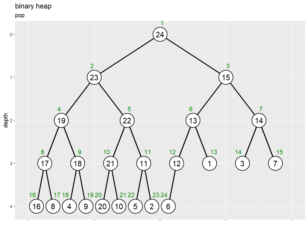
　要素数を指定して、数列を作成します。

# 要素数を指定
N <- 25

# (簡易的に)数列を作成
a <- 1:N
a

##  [1]  1  2  3  4  5  6  7  8  9 10 11 12 13 14 15 16 17 18 19 20 21 22 23 24 25

　N 個の値を作成します。数列のみが与えられている場合は、要素数を N とします。

　数列をヒープ化します。

# ヒープ化
a <- heapify(a)
a

##  [1] 25 23 24 19 22 13 15 17 18 21 11 12  1 14  7 16  8  4  9 20 10  5  2  6  3

　1番目の要素が最大値になります。

　頂点の描画用のデータフレームを作成します。

# ノードの座標を作成
d <- 0.6
vertex_df <- tibble::tibble(
  value = a, 
  index = 1:length(a), 
  depth = floor(log2(index)), # 縦方向のノード位置
  col_idx = index - 2^depth + 1, # 深さごとのノード番号
  coord_x = (col_idx * 2 - 1) * 1/(2^depth * 2), # 横方向のノード位置
  label_offset = dplyr::if_else(
    condition = index%%2 == 0, true = 0.5+d, false = 0.5-d
  ) # ラベル位置を左右にズラす
)
vertex_df

## # A tibble: 25 × 6
##    value index depth col_idx coord_x label_offset
##    <int> <int> <dbl>   <dbl>   <dbl>        <dbl>
##  1    25     1     0       1  0.5            -0.1
##  2    23     2     1       1  0.25            1.1
##  3    24     3     1       2  0.75           -0.1
##  4    19     4     2       1  0.125           1.1
##  5    22     5     2       2  0.375          -0.1
##  6    13     6     2       3  0.625           1.1
##  7    15     7     2       4  0.875          -0.1
##  8    17     8     3       1  0.0625          1.1
##  9    18     9     3       2  0.188          -0.1
## 10    21    10     3       3  0.312           1.1
## # ℹ 15 more rows

　数列とインデックスを格納して、頂点(ノード)の座標を計算します。
　また、ラベル位置の調整用の値を作成します。この例では、インデックスが偶数の場合は左にズラすために0.5以上の値、奇数の場合は右にズラすために0.5以下の値を格納しています。

　辺の描画用のデータフレームを作成します。

# エッジの座標を作成
edge_df <- dplyr::bind_rows(
  # 子ノードの座標
  vertex_df |> 
    dplyr::filter(depth > 0) |> # 根を除去
    dplyr::mutate(
      edge_id   = index, 
      node_type = "childe" # (確認用)
    ), 
  # 親ノードの座標
  vertex_df |> 
    dplyr::filter(depth > 0) |> # 根を除去
    dplyr::mutate(
      edge_id   = index, 
      node_type = "parent", # (確認用)
      depth   = depth - 1, # 縦方向のノード位置
      index   = index %/% 2, 
      col_idx = index - 2^depth + 1, # 深さごとのノード番号
      coord_x = (col_idx * 2 - 1) * 1/(2^depth * 2) # 横方向のノード位置
    )
) |> 
  dplyr::select(!label_offset) |> 
  dplyr::arrange(edge_id, depth)
edge_df

## # A tibble: 48 × 7
##    value index depth col_idx coord_x edge_id node_type
##    <int> <dbl> <dbl>   <dbl>   <dbl>   <int> <chr>    
##  1    23     1     0       1   0.5         2 parent   
##  2    23     2     1       1   0.25        2 childe   
##  3    24     1     0       1   0.5         3 parent   
##  4    24     3     1       2   0.75        3 childe   
##  5    19     2     1       1   0.25        4 parent   
##  6    19     4     2       1   0.125       4 childe   
##  7    22     2     1       1   0.25        5 parent   
##  8    22     5     2       2   0.375       5 childe   
##  9    13     3     1       2   0.75        6 parent   
## 10    13     6     2       3   0.625       6 childe   
## # ℹ 38 more rows

　数列とインデックスを格納して、辺(エッジ)の始点と終点(根を除く各頂点とその親)の座標を計算します。
　線分間が繋がらないように、子のインデックスをエッジIDとして用います。

　ヒープ化した数列をバイナリツリーとして作図します。

# ツリーの高さを取得
max_h <- floor(log2(N))

# 二分木を作図
d <- 0.1
ggplot() + 
  geom_path(data = edge_df, 
            mapping = aes(x = coord_x, y = depth, group = edge_id), 
            linewidth = 1) + # 辺
  geom_point(data = vertex_df, 
             mapping = aes(x = coord_x, y = depth), 
             size = 12, shape = "circle filled", fill = "white", stroke = 1) + # 頂点
  geom_text(data = vertex_df, 
            mapping = aes(x = coord_x, y = depth, label = value), 
            size = 5) + # 値ラベル
  geom_text(data = vertex_df, 
            mapping = aes(x = coord_x, y = depth, label = index, hjust = label_offset), 
            size = 4, vjust = -2, color = "green4") + # 位置ラベル
  scale_x_continuous(labels = NULL, name = "") + 
  scale_y_reverse(breaks = 0:max_h, minor_breaks = FALSE) + 
  coord_cartesian(xlim = c(0, 1), ylim = c(max_h+d, -d)) + 
  labs(title = "binary heap", 
       subtitle = paste0("height = ", max_h), 
       y = "depth")

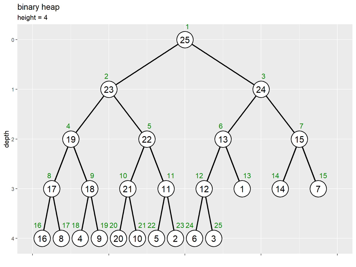
　全ての親子間で親の値が子の値以上であり、根(一番上の頂点)が最大値なのを確認できます。最大値以外の要素がどの頂点(インデックス)なのかは分かりません。

ヒープ化の可視化

　二分ヒープ化のアルゴリズムをグラフで確認します。

　アルゴリズムに従いヒープ化を行って、作図用のデータを作成します。

・作図コード(クリックで展開)

　親子の値の大小関係による要素(値とインデックス)の入れ替えを関数に作成します。

# 親子ノードの入替の実装
swap <- function(value, index, i, N) {
  
  # 数列の値・インデックスを取得
  val_vec <- value
  idx_vec <- index
  
  # 左側の子のインデックスを計算
  child_idx <- i * 2
  
  # 子がなければ終了
  if(child_idx > N) {
    lt <- list(value = val_vec, index = idx_vec, target = i)
    return(lt)
  }
  
  # 値が大きい方の子のインデックスを設定
  if(child_idx+1 <= N & val_vec[child_idx+1] > val_vec[child_idx]) {
    child_idx <- child_idx + 1
  }
  
  # 子が親以下なら終了
  if(val_vec[child_idx] <= val_vec[i]) {
    lt <- list(value = val_vec, index = idx_vec, target = i)
    return(lt)
  }
  
  # 子と親を入替
  val_vec[1:N] <- replace(x = val_vec, list = c(child_idx, i), values = val_vec[c(i, child_idx)])
  idx_vec[1:N] <- replace(x = idx_vec, list = c(child_idx, i), values = idx_vec[c(i, child_idx)])
  
  # 数列を出力
  if(child_idx <= N%/%2) {
    
    # 親子の入替があれば継続
    lt <- list(value = val_vec, index = idx_vec, target = child_idx)
    
  } else {
    
    # 子が葉なら終了
    lt <- list(value = val_vec, index = idx_vec, target = i)
  }
  return(lt)
}

　数列全体と入替範囲のインデックスを受け取り、sub_heapify() と同様に親子の入れ替えを行い、作図用の値を出力します。再帰処理は行いません。
　作図用の値として、「数列の値・インデックス」のベクトルと「入れ替え後のインデックス」の値をリストに格納して出力します。

　要素数を指定して、数列を作成します。

# 要素数を指定
N <- 25

# 数列を作成
a <- sample(x = 1:N, size = N, replace = FALSE)

##  [1] 15  2 12 25 14 10  6 16  7  3 24 23 17 21  1 13  8 22 19  4 20 11  5  9 18

　乱数生成関数 sample() などで数値ベクトルを生成します。

　数列の記録用のデータフレームを作成します。

# 葉を除く頂点数を計算
max_i <- N %/% 2

# 数列を格納
trace_df <- tibble::tibble(
  step  = 0,   # 試行回数
  id    = 1:N, # 元のインデックス
  index = 1:N, # 各試行のインデックス
  value = a    # 要素
) |> 
  dplyr::mutate(
    target_flag = FALSE, # 入替対象の頂点
    heap_flag   = index > max_i # ヒープ化済みの部分木頂点
  )
trace_df

## # A tibble: 25 × 6
##     step    id index value target_flag heap_flag
##    <dbl> <int> <int> <int> <lgl>       <lgl>    
##  1     0     1     1    15 FALSE       FALSE    
##  2     0     2     2     2 FALSE       FALSE    
##  3     0     3     3    12 FALSE       FALSE    
##  4     0     4     4    25 FALSE       FALSE    
##  5     0     5     5    14 FALSE       FALSE    
##  6     0     6     6    10 FALSE       FALSE    
##  7     0     7     7     6 FALSE       FALSE    
##  8     0     8     8    16 FALSE       FALSE    
##  9     0     9     9     7 FALSE       FALSE    
## 10     0    10    10     3 FALSE       FALSE    
## # ℹ 15 more rows

　1データずつ入れ替え処理を行い、数列を記録します。

# 作図用のオブジェクトを初期化
id_vec <- 1:N

# ヒープ化
iter <- 0
for(i in max_i:1) {
  
  # i番目の頂点を設定
  target_idx <- i
  
  # i番目の頂点を根とする部分木をヒープ化
  swap_flag <- TRUE
  while(swap_flag) {
    
    # 試行回数をカウント
    iter <- iter + 1
    
    # 親子の値を比較・入替
    res_lt <- swap(a, id_vec, target_idx, N)
    a[1:N]      <- res_lt[["value"]]
    id_vec[1:N] <- res_lt[["index"]]
    next_target_idx <- res_lt[["target"]]
    
    # 数列を格納
    tmp_df <- tibble::tibble(
      step  = iter, 
      id    = id_vec, 
      index = 1:N, 
      value = a
    ) |> 
      dplyr::mutate(
        target_flag = index %in% c(target_idx, target_idx*2, target_idx*2+1), # 入替対象の親子
        heap_flag   = index >= i & !target_flag # 入替対象を除く処理済み頂点
      )
    
    # 結果を記録
    trace_df <- dplyr::bind_rows(trace_df, tmp_df)
    
    # 入替の有無を確認
    if(target_idx == next_target_idx) {
      
      # 入替がなければ終了
      swap_flag <- FALSE
      
    } else {
      
      # 入替があれば入替後の頂点を親として設定
      target_idx <- next_target_idx
    }
    
    # 途中経過を表示
    #print(paste0("--- step: ", iter, " ---"))
    #print(a)
  }
}

　「ヒープ化の実装」のときと同様にして、要素を入れ替えていきます。再帰処理に関しては、while() を使って入れ替えが行われなくなるまで繰り返します。
　数列 a の初期値のインデックス(1 から N の整数)を id_vec としておき、a の要素の入れ替えに対応するように id_vec の要素も入れ替えます。
　試行ごとに、数列やインデックスをデータフレームに保存します。

　各試行の二分木のグラフを切り替えて推移を確認します。

・作図コード(クリックで展開)

　試行ごとの頂点の描画用のデータフレームを作成します。

# 頂点の座標を作成
trace_vertex_df <- trace_df |> 
  dplyr::mutate(
    depth   = floor(log2(index)), # 縦方向の頂点位置
    col_idx = index - 2^depth + 1, # 深さごとの頂点番号
    coord_x = (col_idx * 2 - 1) * 1/(2^depth * 2), # 横方向の頂点位置
  )
trace_vertex_df

## # A tibble: 550 × 9
##     step    id index value target_flag heap_flag depth col_idx coord_x
##    <dbl> <int> <int> <int> <lgl>       <lgl>     <dbl>   <dbl>   <dbl>
##  1     0     1     1    15 FALSE       FALSE         0       1  0.5   
##  2     0     2     2     2 FALSE       FALSE         1       1  0.25  
##  3     0     3     3    12 FALSE       FALSE         1       2  0.75  
##  4     0     4     4    25 FALSE       FALSE         2       1  0.125 
##  5     0     5     5    14 FALSE       FALSE         2       2  0.375 
##  6     0     6     6    10 FALSE       FALSE         2       3  0.625 
##  7     0     7     7     6 FALSE       FALSE         2       4  0.875 
##  8     0     8     8    16 FALSE       FALSE         3       1  0.0625
##  9     0     9     9     7 FALSE       FALSE         3       2  0.188 
## 10     0    10    10     3 FALSE       FALSE         3       3  0.312 
## # ℹ 540 more rows

　各試行の数列データ trace_df を用いて、試行ごとに(step 列でグループ化して)、「ヒープの可視化」のときと同様にして、頂点の座標を計算します。

　辺の描画用のデータフレームを作成します。

# 辺の座標を作成
edge_df <- dplyr::bind_rows(
  # 子の座標
  trace_vertex_df |> 
    dplyr::filter(step == 0, depth > 0) |> # 1試行分のデータを抽出・根を除去
    dplyr::mutate(
      edge_id = index
    ), 
  # 親の座標
  trace_vertex_df |> 
    dplyr::filter(step == 0, depth > 0) |> # 1試行分のデータを抽出・根を除去
    dplyr::mutate(
      edge_id = index, # 子インデックス
      depth   = depth - 1, # 縦方向の頂点位置
      index   = index %/% 2, # 親インデックス
      col_idx = index - 2^depth + 1, # 深さごとの頂点番号
      coord_x = (col_idx * 2 - 1) * 1/(2^depth * 2) # 横方向の頂点位置
    )
) |> 
  dplyr::select(!step) |> # フレーム遷移の影響から外す
  dplyr::arrange(edge_id, depth)
edge_df

## # A tibble: 48 × 9
##       id index value target_flag heap_flag depth col_idx coord_x edge_id
##    <int> <dbl> <int> <lgl>       <lgl>     <dbl>   <dbl>   <dbl>   <int>
##  1     2     1     2 FALSE       FALSE         0       1   0.5         2
##  2     2     2     2 FALSE       FALSE         1       1   0.25        2
##  3     3     1    12 FALSE       FALSE         0       1   0.5         3
##  4     3     3    12 FALSE       FALSE         1       2   0.75        3
##  5     4     2    25 FALSE       FALSE         1       1   0.25        4
##  6     4     4    25 FALSE       FALSE         2       1   0.125       4
##  7     5     2    14 FALSE       FALSE         1       1   0.25        5
##  8     5     5    14 FALSE       FALSE         2       2   0.375       5
##  9     6     3    10 FALSE       FALSE         1       2   0.75        6
## 10     6     6    10 FALSE       FALSE         2       3   0.625       6
## # ℹ 38 more rows

　1試行分(この例だと初期値)の頂点の座標データを取り出して、「ヒープの可視化」のときと同様にして、辺(始点・終点)の座標を計算します。

　インデックスラベルの描画用のデータフレームを作成します。

# インデックスラベルの座標を作成
d <- 0.6
index_df <- trace_vertex_df |> 
  dplyr::filter(step == 0) |> # 1試行分のデータを抽出
  dplyr::mutate(
    offset = dplyr::if_else(
      condition = index%%2 == 0, true = 0.5+d, false = 0.5-d
    ) # ラベル位置を左右にズラす
  ) |> 
  dplyr::select(!step) # フレーム遷移の影響から外す
index_df

## # A tibble: 25 × 9
##       id index value target_flag heap_flag depth col_idx coord_x offset
##    <int> <int> <int> <lgl>       <lgl>     <dbl>   <dbl>   <dbl>  <dbl>
##  1     1     1    15 FALSE       FALSE         0       1  0.5      -0.1
##  2     2     2     2 FALSE       FALSE         1       1  0.25      1.1
##  3     3     3    12 FALSE       FALSE         1       2  0.75     -0.1
##  4     4     4    25 FALSE       FALSE         2       1  0.125     1.1
##  5     5     5    14 FALSE       FALSE         2       2  0.375    -0.1
##  6     6     6    10 FALSE       FALSE         2       3  0.625     1.1
##  7     7     7     6 FALSE       FALSE         2       4  0.875    -0.1
##  8     8     8    16 FALSE       FALSE         3       1  0.0625    1.1
##  9     9     9     7 FALSE       FALSE         3       2  0.188    -0.1
## 10    10    10     3 FALSE       FALSE         3       3  0.312     1.1
## # ℹ 15 more rows

　1試行分の頂点の座標データを取り出して、「ヒープの可視化」のときと同様にして、ラベル位置の調整値を追加します。

　ヒープ化済みの頂点の描画用のデータフレームを作成します。

# ヒープ化済み頂点の座標を作成
heap_df <- trace_vertex_df |> 
  dplyr::filter(heap_flag, step > 0) |> # ヒープ化済み頂点を抽出・初期値を除去:(表示フレームの調整用)
  dplyr::mutate(
    step = step - 1 # 表示フレームを調整
  ) |> 
  dplyr::bind_rows(
    trace_vertex_df |> 
      dplyr::filter(step == max(step))
  ) # 最終値を追加:(表示フレームの調整用)
heap_df

## # A tibble: 406 × 9
##     step    id index value target_flag heap_flag depth col_idx coord_x
##    <dbl> <int> <int> <int> <lgl>       <lgl>     <dbl>   <dbl>   <dbl>
##  1     0    13    13    17 FALSE       TRUE          3       6  0.688 
##  2     0    14    14    21 FALSE       TRUE          3       7  0.812 
##  3     0    15    15     1 FALSE       TRUE          3       8  0.938 
##  4     0    16    16    13 FALSE       TRUE          4       1  0.0312
##  5     0    17    17     8 FALSE       TRUE          4       2  0.0938
##  6     0    18    18    22 FALSE       TRUE          4       3  0.156 
##  7     0    19    19    19 FALSE       TRUE          4       4  0.219 
##  8     0    20    20     4 FALSE       TRUE          4       5  0.281 
##  9     0    21    21    20 FALSE       TRUE          4       6  0.344 
## 10     0    22    22    11 FALSE       TRUE          4       7  0.406 
## # ℹ 396 more rows

　各試行の頂点の座標データ trace_vertex_df から、各試行におけるヒープ化済み要素の座標データ(heap_flag 列が TRUE の行)を取り出します。
　1試行早く表示するために、step 列を-1し、最終値(全ての要素がヒープ化済み)のデータを複製します。

　入れ替え対象の頂点の描画用のデータフレームを作成します。

# 入替対象の頂点の座標を作成
target_vertex_df <- trace_vertex_df |> 
  dplyr::filter(target_flag) |> # 入替対象の親を抽出
  dplyr::mutate(
    step = step - 1 # 表示フレームを調整
  ) |> 
  dplyr::arrange(step, index)
target_vertex_df

## # A tibble: 63 × 9
##     step    id index value target_flag heap_flag depth col_idx coord_x
##    <dbl> <int> <int> <int> <lgl>       <lgl>     <dbl>   <dbl>   <dbl>
##  1     0    12    12    23 TRUE        FALSE         3       5   0.562
##  2     0    24    24     9 TRUE        FALSE         4       9   0.531
##  3     0    25    25    18 TRUE        FALSE         4      10   0.594
##  4     1    11    11    24 TRUE        FALSE         3       4   0.438
##  5     1    22    22    11 TRUE        FALSE         4       7   0.406
##  6     1    23    23     5 TRUE        FALSE         4       8   0.469
##  7     2    21    10    20 TRUE        FALSE         3       3   0.312
##  8     2    20    20     4 TRUE        FALSE         4       5   0.281
##  9     2    10    21     3 TRUE        FALSE         4       6   0.344
## 10     3    18     9    22 TRUE        FALSE         3       2   0.188
## # ℹ 53 more rows

　各試行における入れ替え対象の座標データ(target_flag 列が TRUE の行)を取り出します。

　入れ替え対象の頂点を結ぶ辺の描画用のデータフレームを作成します。

# 入替対象の辺の座標を作成
target_edge_df <- dplyr::bind_rows(
  # 親の座標
  target_vertex_df |> 
    dplyr::group_by(step) |> 
    dplyr::filter(index == min(index)) |> # 親を抽出
    dplyr::ungroup() |> 
    tidyr::uncount(weights = 2, .id = "childe_id") |> # 子の数に複製
    dplyr::mutate(
      childe_id = childe_id - 1, # 行番号を子IDに変換
      edge_id   = index * 2 + childe_id # 子インデックス
    ) |> 
    dplyr::filter(edge_id <= N), # 子がなければ除去
  # 子の座標
  target_vertex_df |> 
    dplyr::group_by(step) |> 
    dplyr::filter(index != min(index)) |> # 子を抽出
    dplyr::ungroup() |> 
    dplyr::mutate(
      edge_id = index
    )
) |> 
  dplyr::arrange(step, index)
target_edge_df |> 
  dplyr::select(!col_idx) # (資料作成用に間引き)

## # A tibble: 84 × 10
##     step    id index value target_flag heap_flag depth coord_x childe_id edge_id
##    <dbl> <int> <int> <int> <lgl>       <lgl>     <dbl>   <dbl>     <dbl>   <dbl>
##  1     0    12    12    23 TRUE        FALSE         3   0.562         0      24
##  2     0    12    12    23 TRUE        FALSE         3   0.562         1      25
##  3     0    24    24     9 TRUE        FALSE         4   0.531        NA      24
##  4     0    25    25    18 TRUE        FALSE         4   0.594        NA      25
##  5     1    11    11    24 TRUE        FALSE         3   0.438         0      22
##  6     1    11    11    24 TRUE        FALSE         3   0.438         1      23
##  7     1    22    22    11 TRUE        FALSE         4   0.406        NA      22
##  8     1    23    23     5 TRUE        FALSE         4   0.469        NA      23
##  9     2    21    10    20 TRUE        FALSE         3   0.312         0      20
## 10     2    21    10    20 TRUE        FALSE         3   0.312         1      21
## # ℹ 74 more rows

　入れ替え対象の頂点の座標データ target_vertex_df から、入替元の頂点とその子の座標データを取り出して結合します。親のデータは、各試行におけるインデックスが最小の要素(行)で、子の数に対応するように複製します。

　ヒープ化の推移のアニメーションを作成します。

# ヒープ化のアニメーションを作図
max_h <- floor(log2(N))
graph <- ggplot() + 
  geom_path(data = edge_df, 
            mapping = aes(x = coord_x, y = depth, group = edge_id), 
            linewidth = 1) + # 辺
  geom_path(data = target_edge_df,
            mapping = aes(x = coord_x, y = depth, group = edge_id),
            color = "red", linewidth = 1, linetype = "dashed") + # 入替対象の辺
  geom_point(data = target_vertex_df,
             mapping = aes(x = coord_x, y = depth, group = step),
             size = 14, color = "red", alpha = 0.5) + # 入替対象の頂点
  geom_point(data = heap_df,
             mapping = aes(x = coord_x, y = depth, group = step),
             size = 14, color = "blue", alpha = 0.5) + # ヒープ化済みの頂点
  geom_point(data = trace_vertex_df, 
             mapping = aes(x = coord_x, y = depth, group = id), 
             size = 12, shape = "circle filled", fill = "white", stroke = 1) + # 頂点
  geom_text(data = trace_vertex_df, 
            mapping = aes(x = coord_x, y = depth, label = as.character(value), group = id), 
            size = 5) + # 値ラベル
  geom_text(data = index_df, 
            mapping = aes(x = coord_x, y = depth, label = index, hjust = offset), 
            size = 4, vjust = -1.7, color = "green4") + # インデックスラベル
  gganimate::transition_states(states = step, transition_length = 9, state_length = 1, wrap = FALSE) + # フレーム遷移
  gganimate::ease_aes("cubic-in-out") + # 遷移の緩急
  scale_x_continuous(labels = NULL) + 
  scale_y_reverse(breaks = 0:max_h, minor_breaks = FALSE) + 
  coord_cartesian(xlim = c(0, 1)) + 
  labs(title = "heapify", 
       subtitle = "step: {next_state}", 
       x = "", y = "depth")

# フレーム数を取得
frame_num <- max(trace_df[["step"]]) + 1

# 遷移フレーム数を指定
s <- 20

# gif画像を作成
gganimate::animate(
  plot = graph, 
  nframes = (frame_num + 2)*s, start_pause = s, end_pause = s, fps = 20, 
  width = 1200, height = 600, 
  renderer = gganimate::gifski_renderer()
)

　transition_states() のフレーム制御の引数 states に試行回数列 step を指定して、これまでと同様に作図します。
　animate() の plot 引数にグラフオブジェクト、nframes 引数にフレーム数を指定して、gif画像を作成します。
　初期値を含むため試行回数は最大値+1です。transition_states() でアニメーションを作成すると、フレーム間の値を補完して、状態の遷移を描画します。遷移(1試行当たり)のフレーム数を s として、試行回数の s 倍の値を nframes 引数に指定します。

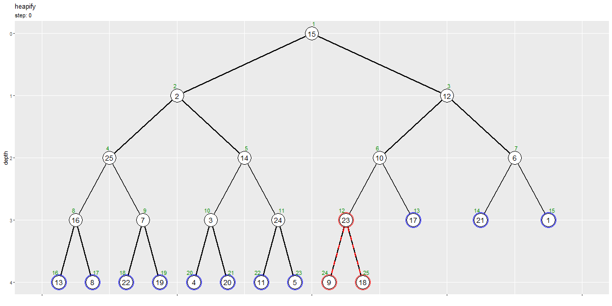
　入れ替え対象の頂点を赤色、親子がヒープ化済みの頂点を青色の塗りつぶしで示します。

　葉(子の無い頂点)を除く一番後の頂点(N番目の頂点の親)から順番に、各頂点を根として部分木をヒープ化していきます。
　部分木の根の値を子と比較して、子の方が大きければ入れ替えます。入れ替えた場合はさらに、入替先の子(元の位置からだと孫)と比較して、子の方が大きければ入れ替える操作を繰り返します。入れ替えが行われなかった場合は、次の頂点に移ります。
　「根より子の方が小さい」または「根が葉まで到達する」と、部分木がヒープ化された状態になります。この操作を後から繰り返すことで、末端の(小さな)部分木から徐々に、全体がヒープ化されるのを確認できます。

　ここでの試行回数(stepの値)は、この可視化方法における試行番号(作図処理上の値)であり他の手法と対応していません。

値の挿入

　次は、ヒープに新たな値を追加する操作の実装と可視化を行います。

値の挿入の実装

　二分ヒープへの値の挿入のアルゴリズムを関数として実装します。

　値の挿入を実装します。

# 値の挿入の実装
push <- function(vec, val) {
  
  # 挿入要素(子)のインデックスを設定
  i <- length(vec) + 1
  
  # ヒープ化
  while(i > 1) { # (根に達するまで)
    
    # 親のインデックスを計算
    parent_idx <- i %/% 2
    
    # 親が子以上なら終了
    if(vec[parent_idx] >= val) break
    
    # 子と親を入替
    vec[i] <- vec[parent_idx] # 親の値を子の位置に移動
    i      <- parent_idx      # 挿入位置を親の位置に更新
  }
  
  # 値を挿入
  vec[i] <- val
  
  # 数列を出力
  return(vec)
}

　ヒープ化済みの数列を vec、挿入する値を val、値の挿入位置(インデックス)を i とします。
　i の初期値として挿入後の要素数を設定します。この操作が、末尾への要素の挿入に対応します。
　i 番目の頂点(要素)の親のインデックスを parent_idx として計算します。頂点 $v_i$ の親 $v_j$ のインデックスは $j = \lfloor \frac{i}{2} \rfloor$ で求まります。

　挿入する値 val と親の値 vec[parent_idx] を大小比較していき、挿入位置 i を探索します。
　挿入する値が大きければ、vec の parent_idx 番目の値を i 番目に複製し、挿入位置 i を parent_idx に更新します。この操作が、親子要素の入れ替えに対応します。ただしこの時点では、vec の i, parent_idx 番目が同じ値です。
　「親の値が挿入値以上」または「挿入位置が根(親がない)」であれば、ループ処理を終了して vec の i 番目に val を代入します。この操作によって入れ替えが完了します。

　アルゴリズムの詳しい解説は、本のcode 10.5(前半)などを参照してください。

　実装した関数を試してみます。

　ヒープを作成して、値を挿入します。

# 要素数を指定
N <- 25

# (簡易的に)数列を作成
a <- 1:N

# ヒープ化
a <- heapify(a)

# 挿入値を指定
x <- 23.5

# 値を挿入してヒープ化
a <- push(a, x)
a; length(a)

##  [1] 25.0 23.0 24.0 19.0 22.0 23.5 15.0 17.0 18.0 21.0 11.0 12.0 13.0 14.0  7.0
## [16] 16.0  8.0  4.0  9.0 20.0 10.0  5.0  2.0  6.0  3.0  1.0
## [1] 26

　要素数が1つ増えます。

　「ヒープの可視化」のときのコードで、新たな値を追加したヒープをバイナリツリーで確認します。

　「ヒープの可視化」のときの図から、この図に変化します。

値の挿入の可視化

　続いて、二分ヒープ化への値の挿入のアルゴリズムをグラフで確認します。

　アルゴリズムに従いヒープ化を行って、作図用のデータを作成します。

・作図コード(クリックで展開)

　要素数を指定して、ヒープを作成します。

# 要素数を指定
initial_N <- 40

# ヒープを作成
initial_a <- sample(x = 1:initial_N, size = initial_N, replace = FALSE) |> 
  heapify()
initial_a

##  [1] 40 39 38 37 28 29 33 35 36 18 20 25 27 16 26 32 24 34 30 13  4 17  2  3 10
## [26]  7  1 15 12  8 21  6 31 14 19  5 22  9 23 11

　N - 1 個の値を作成して、heapify() でヒープ化します。

　値を指定して、ヒープに挿入します。

# 挿入する値を指定
x <- 38.5

# 値を挿入
a <- c(initial_a, x)

# 挿入後の要素数を取得
N <- length(a)
a; N

##  [1] 40.0 39.0 38.0 37.0 28.0 29.0 33.0 35.0 36.0 18.0 20.0 25.0 27.0 16.0 26.0
## [16] 32.0 24.0 34.0 30.0 13.0  4.0 17.0  2.0  3.0 10.0  7.0  1.0 15.0 12.0  8.0
## [31] 21.0  6.0 31.0 14.0 19.0  5.0 22.0  9.0 23.0 11.0 38.5
## [1] 41

　ヒープ(数列)の末尾に値を追加します。

　数列の記録用のデータフレームを作成します。

# 数列を格納
trace_df <- dplyr::bind_rows(
  # 初期値
  tibble::tibble(
    step  = 0, 
    id    = 1:initial_N, 
    index = id, 
    value = initial_a, 
    target_flag = FALSE
  ), 
  # 挿入後
  tibble::tibble(
    step  = 1, 
    id    = 1:N, 
    index = id, 
    value = a, 
    target_flag = index == N # 挿入対象
  )
)
trace_df

## # A tibble: 81 × 5
##     step    id index value target_flag
##    <dbl> <int> <int> <dbl> <lgl>      
##  1     0     1     1    40 FALSE      
##  2     0     2     2    39 FALSE      
##  3     0     3     3    38 FALSE      
##  4     0     4     4    37 FALSE      
##  5     0     5     5    28 FALSE      
##  6     0     6     6    29 FALSE      
##  7     0     7     7    33 FALSE      
##  8     0     8     8    35 FALSE      
##  9     0     9     9    36 FALSE      
## 10     0    10    10    18 FALSE      
## # ℹ 71 more rows

　初期値(挿入前)と挿入後の数列をデータフレームに格納します。

　1試行ずつ入れ替え処理を行い、数列を記録します。

# 挿入要素のインデックスを設定
i <- N

# 作図用のオブジェクトを初期化
id_vec <- 1:N

# ヒープ化
iter <- 1
break_flag <- FALSE
while(i > 1) {
  
  # 試行回数を更新
  iter <- iter + 1
  
  # 親のインデックスを計算
  parent_idx <- i %/% 2
  
  # 親のインデックスを計算
  parent_idx <- i %/% 2
  
  # 親が子未満なら親子を入替
  if(a[parent_idx] < a[i]) {
    a[1:N]      <- replace(x = a, list = c(i, parent_idx), values = a[c(parent_idx, i)])
    id_vec[1:N] <- replace(x = id_vec, list = c(i, parent_idx), values = id_vec[c(parent_idx, i)])
  } else {
    break_flag <- TRUE
  }
  
  # 数列を格納
  tmp_df <- tibble::tibble(
    step  = iter, 
    id    = id_vec, 
    index = 1:N, 
    value = a, 
    target_flag = index %in% c(i, parent_idx) # 入替対象
  )
  
  # 数列を記録
  trace_df <- dplyr::bind_rows(trace_df, tmp_df)

  # 親が子以上なら終了
  if(break_flag) break
  
  # 挿入位置を親の位置に更新
  i <- parent_idx
  
  # 途中経過を表示
  #print(paste0("--- step: ", iter, " ---"))
  #print(a)
}

　「値の挿入の実装」のときと同様にして要素を入れ替えていき、試行ごとに数列やインデックスをデータフレームに保存します。

　各試行の二分木のグラフを切り替えて推移を確認します。

・作図コード(クリックで展開)

　「ヒープ化の可視化」のときのコードで、試行ごとの頂点と辺、インデックラベルの描画用のデータフレーム(trace_vertex_df・edge_df・index_df)を作成します。ただし、初期値(step 列が 0)ではなく、挿入後(step 列が 1 などの値)の座標データを取り出します。

　入れ替え対象の頂点と辺の描画用のデータフレームを作成します。

# 入替対象の頂点の座標を作成
target_vertex_df <- trace_vertex_df |> 
  dplyr::filter(target_flag) |> # 入替対象の親を抽出
  dplyr::mutate(
    step = step - 1 # 表示フレームを調整
  ) |> 
  dplyr::arrange(step, index)

# 入替対象の辺の座標を作成
target_edge_df <- target_vertex_df |> 
  dplyr::bind_rows(
    target_vertex_df |> 
      dplyr::filter(step == 0)
  ) # (警告文回避用に挿入値を複製)
target_edge_df

## # A tibble: 10 × 8
##     step    id index value target_flag depth col_idx coord_x
##    <dbl> <int> <int> <dbl> <lgl>       <dbl>   <dbl>   <dbl>
##  1     0    41    41  38.5 TRUE            5      10   0.297
##  2     1    41    20  38.5 TRUE            4       5   0.281
##  3     1    20    41  13   TRUE            5      10   0.297
##  4     2    41    10  38.5 TRUE            3       3   0.312
##  5     2    10    20  18   TRUE            4       5   0.281
##  6     3    41     5  38.5 TRUE            2       2   0.375
##  7     3     5    10  28   TRUE            3       3   0.312
##  8     4     2     2  39   TRUE            1       1   0.25 
##  9     4    41     5  38.5 TRUE            2       2   0.375
## 10     0    41    41  38.5 TRUE            5      10   0.297

　「ヒープ化の可視化」のときのコードで trace_vertex_df を作成します。
　値の挿入操作では1点の座標データしかないので、挿入時(値を調整したので step 列が 0 の行)を複製して target_edge_df とします。または、挿入時のデータ(行)を取り除いて、座標データを欠損させた step 列が 0 の行を追加します(追加しておかないと(?)フレームの表示順がバグります)。

　ヒープに値を挿入した際の推移のアニメーションを作成します。

# ヒープ化のアニメーションを作図
max_h <- floor(log2(N))
graph <- ggplot() + 
  geom_path(data = edge_df,
            mapping = aes(x = coord_x, y = depth, group = edge_id),
            linewidth = 1) + # 辺
  geom_path(data = target_edge_df,
            mapping = aes(x = coord_x, y = depth, group = step),
            color = "red", linewidth = 1, linetype = "dashed") + # 入替対象の辺
  geom_point(data = target_vertex_df,
             mapping = aes(x = coord_x, y = depth, group = step),
             size = 14, color = "red", alpha = 0.5) + # 入替対象の頂点
  geom_point(data = trace_vertex_df,
             mapping = aes(x = coord_x, y = depth, group = id),
             size = 12, shape = "circle filled", fill = "white", stroke = 1) + # 頂点
  geom_text(data = trace_vertex_df,
            mapping = aes(x = coord_x, y = depth, label = as.character(value), group = id),
            size = 5) + # 値ラベル
  geom_text(data = index_df,
            mapping = aes(x = coord_x, y = depth, label = index, hjust = offset),
            size = 4, vjust = -1.7, color = "green4") + # インデックスラベル
  gganimate::transition_states(states = step, transition_length = 9, state_length = 1, wrap = FALSE) + # フレーム遷移
  gganimate::ease_aes("cubic-in-out") + # 遷移の緩急
  scale_x_continuous(labels = NULL) + 
  scale_y_reverse(breaks = 0:max_h, minor_breaks = FALSE) + 
  coord_cartesian(xlim = c(0, 1)) + 
  labs(title = "heapify : push (up-heap)", 
       subtitle = "step: {next_state}", 
       x = "", y = "depth")

# フレーム数を取得
frame_num <- max(trace_df[["step"]]) + 1

# 遷移フレーム数を指定
s <- 20

# gif画像を作成
gganimate::animate(
  plot = graph, 
  nframes = (frame_num + 2)*s, start_pause = s, end_pause = s, fps = 20, 
  width = 1200, height = 600, 
  renderer = gganimate::gifski_renderer()
)

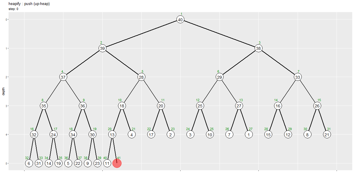
　挿入対象または入替対象の頂点を赤色の塗りつぶしで示します。

　ヒープ化されている元の要素数を $N$ とすると、 $N + 1$ 番目の頂点(要素)に値を追加します。ヒープ条件を満たさなくなる場合があるので、追加した値と親の値を比較・入替を繰り返します。
　ヒープ条件を満たすまで、挿入値とその親を入れ替えていくことでヒープ化されるのを確認できます。

ヒープ化の可視化

　「ヒープ化」では、数列自体をヒープとして値の入れ替えを行いました。ここでは、数列の値を1つずつヒープに挿入していく場合のアルゴリズムをグラフで確認します。

　アルゴリズムに従いヒープ化を行って、作図用のデータを作成します。

・作図コード(クリックで展開)

　要素数を指定して、数列を作成します。

# 要素数を指定
N <- 25

# 数列を作成
initial_a <- sample(x = 1:N, size = N, replace = FALSE)
initial_a

##  [1] 15  2 12 25 14 10  6 16  7  3 24 23 17 21  1 13  8 22 19  4 20 11  5  9 18

　数列の記録用のデータフレームを作成します。

# 1番目の要素を挿入
a <- initial_a[1]

# 数列を格納
trace_df <- tibble::tibble(
  step  = 0, # 試行番号
  id    = 1:N, # 元のインデックス
  index = c(1, rep(NA, times = N-1)), # 試行ごとのインデックス:(未挿入はNAとする)
  value = initial_a, # 要素:(未挿入要素も含める)
  target_flag = FALSE, # 挿入・入替対象:(初手FALSEの方が処理が楽)
  insert_flag = !is.na(index) # 挿入済み要素
)
trace_df

## # A tibble: 25 × 6
##     step    id index value target_flag insert_flag
##    <dbl> <int> <dbl> <int> <lgl>       <lgl>      
##  1     0     1     1    15 FALSE       TRUE       
##  2     0     2    NA     2 FALSE       FALSE      
##  3     0     3    NA    12 FALSE       FALSE      
##  4     0     4    NA    25 FALSE       FALSE      
##  5     0     5    NA    14 FALSE       FALSE      
##  6     0     6    NA    10 FALSE       FALSE      
##  7     0     7    NA     6 FALSE       FALSE      
##  8     0     8    NA    16 FALSE       FALSE      
##  9     0     9    NA     7 FALSE       FALSE      
## 10     0    10    NA     3 FALSE       FALSE      
## # ℹ 15 more rows

　1番目の要素を挿入した状態を初期値とします。初回は要素が1つなので入れ替えは不要です。

　1データずつ挿入と入れ替え処理を行い、数列を記録します。

# 作図用のオブジェクトを初期化
id_vec <- 1:N

# 値の挿入とヒープ化
iter <- 0
for(n in 2:N) {
  
  # 末尾に要素を追加
  a <- c(a, initial_a[n])
  i <- n
  
  # 要素を追加した数列を格納
  tmp_df <- tibble::tibble(
    step  = iter + 0.5, # (挿入操作は0.5とする)
    id    = id_vec, 
    index = c(1:n, rep(NA, times = N-n)), 
    value = c(a, initial_a[(n+1):N])[1:N], 
    target_flag = index %in% i, # 挿入対象
    insert_flag = !is.na(index)
  )
  
  # 数列を記録
  trace_df <- dplyr::bind_rows(trace_df, tmp_df)
  
  # ヒープ化
  break_flag <- FALSE
  while(i > 1) {
    
    # 試行回数を更新
    iter <- iter + 1
    
    # 親のインデックスを計算
    parent_idx <- i %/% 2
    
    # 親が子未満なら親子を入替
    if(a[parent_idx] < a[i]) {
      a[1:n]      <- replace(x = a, list = c(i, parent_idx), values = a[c(parent_idx, i)])
      id_vec[1:n] <- replace(x = id_vec[1:n], list = c(i, parent_idx), values = id_vec[c(parent_idx, i)])
    } else {
      break_flag <- TRUE
    }
    
    # 要素を入れ替えた数列を格納
    tmp_df <- tibble::tibble(
      step  = iter, # (入替操作は1とする)
      id    = id_vec, 
      index = c(1:n, rep(NA, times = N-n)), 
      value = c(a, initial_a[(n+1):N])[1:N], 
      target_flag = index %in% c(i, parent_idx), # 入替対象
      insert_flag = !is.na(index)
    )
    
    # 数列を記録
    trace_df <- dplyr::bind_rows(trace_df, tmp_df)
    
    # 親が子以上なら終了
    if(break_flag) break
    
    # 挿入位置を親の位置に更新
    i <- parent_idx
    
    # 途中経過を表示
    #print(paste0("--- step: ", iter, " ---"))
    #print(a)
  }
}

　値の挿入時と要素の比較・入替時に、数列やインデックスをデータフレームに保存します。要素の入れ替えが行われなかった場合も数列を記録します。
　この例では、挿入時の試行回数のカウントを0.5とします。（挿入時も1でカウントした方が作図処理が簡単ですが、「ヒープ化の可視化」の図と比較する際に、値の大小比較回数を比べるためです。）　各試行における未挿入要素もデータフレームに格納しておき、insert_flag 列で区別します。

　各試行の二分木のグラフを切り替えて推移を確認します。

・作図コード(クリックで展開)

　試行ごとの頂点の描画用のデータフレームを作成します。

# 未挿入要素のプロット位置を設定
max_y <- floor(log2(N)) + 1

# 頂点の座標を作成
trace_vertex_df <- dplyr::bind_rows(
  # 挿入済み要素の座標
  trace_df |> 
    dplyr::filter(insert_flag) |> # 挿入済み要素を抽出
    dplyr::mutate(
      depth   = floor(log2(index)), # 縦方向の頂点位置
      col_idx = index - 2^depth + 1, # 深さごとの頂点番号
      coord_x = (col_idx * 2 - 1) * 1/(2^depth * 2), # 横方向の頂点位置
    ), 
  # 未挿入要素の座標
  trace_df |> 
    dplyr::filter(!insert_flag) |> # 未挿入要素を抽出
    dplyr::mutate(
      depth = max_y, # 縦方向の頂点位置
      coord_x = id / (N + 1) # 横方向の頂点位置
    )
) |> 
  dplyr::arrange(step, index)
trace_vertex_df

## # A tibble: 1,675 × 9
##     step    id index value target_flag insert_flag depth col_idx coord_x
##    <dbl> <int> <dbl> <int> <lgl>       <lgl>       <dbl>   <dbl>   <dbl>
##  1     0     1     1    15 FALSE       TRUE            0       1  0.5   
##  2     0     2    NA     2 FALSE       FALSE           5      NA  0.0769
##  3     0     3    NA    12 FALSE       FALSE           5      NA  0.115 
##  4     0     4    NA    25 FALSE       FALSE           5      NA  0.154 
##  5     0     5    NA    14 FALSE       FALSE           5      NA  0.192 
##  6     0     6    NA    10 FALSE       FALSE           5      NA  0.231 
##  7     0     7    NA     6 FALSE       FALSE           5      NA  0.269 
##  8     0     8    NA    16 FALSE       FALSE           5      NA  0.308 
##  9     0     9    NA     7 FALSE       FALSE           5      NA  0.346 
## 10     0    10    NA     3 FALSE       FALSE           5      NA  0.385 
## # ℹ 1,665 more rows

　「ヒープ化の可視化」のときと同様に作成した挿入済み(ヒープ化対象)要素の座標データと、未挿入要素の座標データを作成して結合します。未挿入要素のプロット位置を max_y とします。

　試行ごとの辺の描画用のデータフレームを作成します。

# 辺の座標を作成
trace_edge_df <- dplyr::bind_rows(
  # 子の座標
  trace_vertex_df |> 
    dplyr::filter(insert_flag, step > 0, depth > 0) |> # 挿入済み要素を抽出、初期値・根を除去
    dplyr::mutate(
      edge_id    = index, 
      edge_label = paste0("step: ", step, ", edge: ", edge_id) # フレームごとに描画用
    ), 
  # 親の座標
  trace_vertex_df |> 
    dplyr::filter(insert_flag, step > 0, depth > 0) |> # 挿入済み要素を抽出、初期値・根を除去
    dplyr::mutate(
      edge_id    = index, # 子インデックス
      edge_label = paste0("step: ", step, ", edge: ", edge_id), # フレームごとに描画用
      depth   = depth - 1, # 縦方向の頂点位置
      index   = index %/% 2, # 親インデックス
      col_idx = index - 2^depth + 1, # 深さごとの頂点番号
      coord_x = (col_idx * 2 - 1) * 1/(2^depth * 2) # 横方向の頂点位置
    ), 
  tibble::tibble(
    step = 0
  ) # (フレーム順の謎バグ回避用)
) |> 
  dplyr::arrange(step, edge_id, index)
trace_edge_df |> 
  dplyr::select(!c(col_idx, coord_x)) # (資料作成用に間引き)

## # A tibble: 1,717 × 9
##     step    id index value target_flag insert_flag depth edge_id edge_label     
##    <dbl> <int> <dbl> <int> <lgl>       <lgl>       <dbl>   <dbl> <chr>          
##  1   0      NA    NA    NA NA          NA             NA      NA <NA>           
##  2   0.5     2     1     2 TRUE        TRUE            0       2 step: 0.5, edg…
##  3   0.5     2     2     2 TRUE        TRUE            1       2 step: 0.5, edg…
##  4   1       2     1     2 TRUE        TRUE            0       2 step: 1, edge:…
##  5   1       2     2     2 TRUE        TRUE            1       2 step: 1, edge:…
##  6   1.5     2     1     2 FALSE       TRUE            0       2 step: 1.5, edg…
##  7   1.5     2     2     2 FALSE       TRUE            1       2 step: 1.5, edg…
##  8   1.5     3     1    12 TRUE        TRUE            0       3 step: 1.5, edg…
##  9   1.5     3     3    12 TRUE        TRUE            1       3 step: 1.5, edg…
## 10   2       2     1     2 FALSE       TRUE            0       2 step: 2, edge:…
## # ℹ 1,707 more rows

　段階的に増える頂点(要素)の数に応じて、辺の座標を作成します。

　インデックスラベルの描画用のデータフレームを作成します。

# インデックスラベルの座標を作成
d <- 0.6
index_df <- trace_vertex_df |> 
  dplyr::filter(insert_flag, step == max(step)) |> # 挿入済み要素・1試行分のデータを抽出
  dplyr::mutate(
    offset = dplyr::if_else(
      condition = index%%2 == 0, true = 0.5+d, false = 0.5-d
    ) # ラベル位置を左右にズラす
  ) |> 
  dplyr::select(!step) # フレーム遷移の影響から外す
index_df

## # A tibble: 25 × 9
##       id index value target_flag insert_flag depth col_idx coord_x offset
##    <int> <dbl> <int> <lgl>       <lgl>       <dbl>   <dbl>   <dbl>  <dbl>
##  1     4     1    25 FALSE       TRUE            0       1  0.5      -0.1
##  2    11     2    24 FALSE       TRUE            1       1  0.25      1.1
##  3    12     3    23 TRUE        TRUE            1       2  0.75     -0.1
##  4    18     4    22 FALSE       TRUE            2       1  0.125     1.1
##  5    21     5    20 FALSE       TRUE            2       2  0.375    -0.1
##  6    25     6    18 TRUE        TRUE            2       3  0.625     1.1
##  7    14     7    21 FALSE       TRUE            2       4  0.875    -0.1
##  8    16     8    13 FALSE       TRUE            3       1  0.0625    1.1
##  9    19     9    19 FALSE       TRUE            3       2  0.188    -0.1
## 10     8    10    16 FALSE       TRUE            3       3  0.312     1.1
## # ℹ 15 more rows

　「ヒープ化の可視化」のときと同様に処理します。ただし、こちらは最終結果(全ての要素がヒープに挿入された試行)の座標データを取り出して使います。

　挿入対象と入れ替え対象の頂点の描画用のデータフレームを作成します。

# 試行番号を取得
step_vec <- unique(trace_df[["step"]])

# 入替対象の頂点の座標を作成
target_vertex_df <- trace_vertex_df |> 
  dplyr::filter(target_flag) |> # 挿入・入替対象を抽出
  dplyr::mutate(
    frame_id = dplyr::dense_rank(step), # 試行回数の抽出用
    step     = step_vec[frame_id] # 表示フレームを調整
  ) |> 
  dplyr::arrange(step, index)
target_vertex_df |> 
  dplyr::select(!c(col_idx, coord_x)) # (資料作成用に間引き)

## # A tibble: 108 × 8
##     step    id index value target_flag insert_flag depth frame_id
##    <dbl> <int> <dbl> <int> <lgl>       <lgl>       <dbl>    <int>
##  1   0       2     2     2 TRUE        TRUE            1        1
##  2   0.5     1     1    15 TRUE        TRUE            0        2
##  3   0.5     2     2     2 TRUE        TRUE            1        2
##  4   1       3     3    12 TRUE        TRUE            1        3
##  5   1.5     1     1    15 TRUE        TRUE            0        4
##  6   1.5     3     3    12 TRUE        TRUE            1        4
##  7   2       4     4    25 TRUE        TRUE            2        5
##  8   2.5     4     2    25 TRUE        TRUE            1        6
##  9   2.5     2     4     2 TRUE        TRUE            2        6
## 10   3       4     1    25 TRUE        TRUE            0        7
## # ℹ 98 more rows

　各試行の頂点の座標データ trace_vertex_df から、各試行における挿入対象または入れ替え対象の要素の座標データ(target_flag 列が TRUE の行)を取り出します。
　1試行早く表示するために、step 列の値を1つ前の値に置き換えます。（挿入時は試行番号を0.5刻みでカウントしているので-1では意図通りに描画されません。）

　入れ替え対象の頂点を結ぶ辺の描画用のデータフレームを作成します。

# 入替対象の辺の座標を作成
target_edge_df <- trace_vertex_df |> 
  dplyr::filter(target_flag) |> # 挿入・入替対象を抽出
  dplyr::mutate(
    frame_id = dplyr::dense_rank(step), # 試行回数の抽出用
  ) |> 
  dplyr::filter(step%%1 == 0) |> # 入替対象を抽出(挿入対象を除去)
  dplyr::group_by(step) |> # 辺IDの作成用
  dplyr::mutate(
    edge_label = paste0("step: ", step, ", id: ", min(index)) # 線分間の干渉回避用
  ) |> 
  dplyr::ungroup() |> 
  dplyr::mutate(
    step = step_vec[frame_id] # 表示フレームを調整
  ) |> 
  dplyr::arrange(step, index)
target_edge_df |> 
  dplyr::select(!c(col_idx, coord_x)) # (資料作成用に間引き)

## # A tibble: 84 × 9
##     step    id index value target_flag insert_flag depth frame_id edge_label    
##    <dbl> <int> <dbl> <int> <lgl>       <lgl>       <dbl>    <int> <chr>         
##  1   0.5     1     1    15 TRUE        TRUE            0        2 step: 1, id: 1
##  2   0.5     2     2     2 TRUE        TRUE            1        2 step: 1, id: 1
##  3   1.5     1     1    15 TRUE        TRUE            0        4 step: 2, id: 1
##  4   1.5     3     3    12 TRUE        TRUE            1        4 step: 2, id: 1
##  5   2.5     4     2    25 TRUE        TRUE            1        6 step: 3, id: 2
##  6   2.5     2     4     2 TRUE        TRUE            2        6 step: 3, id: 2
##  7   3       4     1    25 TRUE        TRUE            0        7 step: 4, id: 1
##  8   3       1     2    15 TRUE        TRUE            1        7 step: 4, id: 1
##  9   4.5     1     2    15 TRUE        TRUE            1        9 step: 5, id: 2
## 10   4.5     5     5    14 TRUE        TRUE            2        9 step: 5, id: 2
## # ℹ 74 more rows

　試行ID(試行回数に対する通し番号)を割り当ててから、挿入時のデータ(step 列が小数点以下の値を持つ行)を取り除いて、試行回数(フレーム用の値)を1つ前の値に置き換えます。

　値の挿入とヒープ化の推移のアニメーションを作成します。

# ヒープ化のアニメーションを作図
graph <- ggplot() + 
  geom_rect(mapping = aes(xmin = 0, xmax = 1, ymin = max_y-0.25, ymax = max_y+0.2), 
            fill = "orange", color = "orange", alpha = 0.1, linetype ="dashed") + # 数列枠
  geom_path(data = trace_edge_df,
            mapping = aes(x = coord_x, y = depth, group = edge_label),
            linewidth = 1) + # 辺
  geom_path(data = target_edge_df,
            mapping = aes(x = coord_x, y = depth, group = edge_label),
            color = "red", linewidth = 1, linetype = "dashed") + # 入替対象の辺
  geom_point(data = target_vertex_df,
             mapping = aes(x = coord_x, y = depth, group = step),
             size = 14, color = "red", alpha = 0.5) + # 挿入・入替対象の頂点
  geom_point(data = trace_vertex_df,
             mapping = aes(x = coord_x, y = depth, group = id),
             size = 12, shape = "circle filled", fill = "white", stroke = 1) + # 頂点
  geom_text(data = trace_vertex_df,
            mapping = aes(x = coord_x, y = depth, label = as.character(value), group = id),
            size = 5) + # 値ラベル
  geom_text(data = index_df,
            mapping = aes(x = coord_x, y = depth, label = index, hjust = offset),
            size = 4, vjust = -1.7, color = "green4") + # インデックスラベル:(ツリー用)
  geom_text(data = index_df,
            mapping = aes(x = index/(N+1), y = max_y, label = index),
            size = 4, hjust = 1.1, vjust = -1.7, color = "green4") + # インデックスラベル:(数列用)
  gganimate::transition_states(states = step, transition_length = 9, state_length = 1, wrap = FALSE) + # フレーム遷移
  gganimate::ease_aes("cubic-in-out") + # 遷移の緩急
  scale_x_continuous(labels = NULL) + 
  scale_y_reverse(breaks = 0:max_y, labels = c(as.character(0:(max_y-1)), ""), minor_breaks = FALSE) + 
  coord_cartesian(xlim = c(0, 1), ylim = c(max_y, 0)) + 
  labs(title = "heapify", 
       subtitle = "step: {next_state}", 
       x = "", y = "depth")

# フレーム数を取得
frame_num <- trace_df[["step"]] |> 
  unique() |> 
  length()

# 遷移フレーム数を指定
s <- 20

# gif画像を作成
gganimate::animate(
  plot = graph, 
  nframes = (frame_num + 2)*s, start_pause = s, end_pause = s, fps = 20, 
  width = 1200, height = 700, 
  renderer = gganimate::gifski_renderer()
)

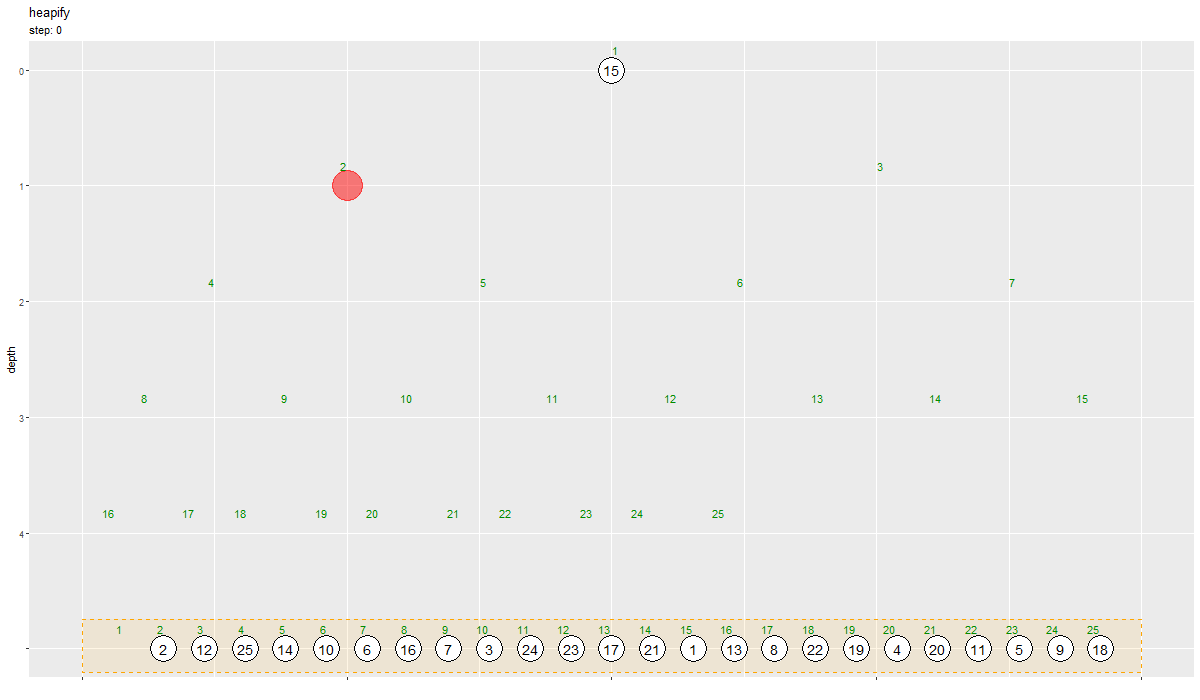
　挿入対象または入替対象の頂点を赤色の丸、未挿入の要素をオレンジ色の枠の塗りつぶしで示します。

　数列の要素を1つずつヒープの末尾に挿入して、それぞれヒープ条件を満たすまで挿入値とその親を入れ替えていくことで、数列全体がヒープ化されるのを確認できます。
　数列全体をヒープとして用いた場合と比べて、ヒープ用のオブジェクト(メモリ)が必要で、操作の回数が増えるのを確認できます。

最大値の削除

　最後は、ヒープの最大値を削除する操作の実装と可視化を行います。

最大値の削除の実装

　二分ヒープの最大値の削除のアルゴリズムを関数として実装します。

　最大値の削除を実装します。

# 最大値の削除の実装
pop <- function(vec) {
  
  # 削除後の要素数を取得
  N <- length(vec) - 1
  
  # 末尾(挿入要素)の値を取得
  val <- vec[N+1]
  
  # 末尾の値を削除
  vec <- vec[-(N+1)]
  
  # 根(親)のインデックスを設定
  i <- 1
  
  # ヒープ化
  while(i*2 <= N) { # (葉に達するまで)
    
    # 左側の子のインデックスを計算
    child_idx <- i * 2
    
    # 値が大きい方の子のインデックスを設定
    if(child_idx+1 <= N & vec[child_idx+1] > vec[child_idx]) { # (&の左がFALSEだと右が処理されずNAにならない)
      child_idx <- child_idx + 1
    }
    
    # 子が親以下なら終了
    if(vec[child_idx] <= val) break
    
    # 親と子を入替
    vec[i] <- vec[child_idx] # 子の値を親の位置に移動
    i      <- child_idx      # 挿入位置を子の位置に更新
  }
  
  # 値を挿入
  vec[i] <- val
  
  # 数列を出力
  return(vec)
}

　ヒープ化済みの数列を vec、削除後の要素数を N、挿入する値(末尾の値)を val、値の挿入位置(インデックス)を i とします。
　vec の(先頭ではなく)末尾の要素を削除して、i の初期値として先頭(最大値)のインデックスを設定します。この操作が、最大値の削除と、末尾の要素の先頭への挿入に対応します。
　i 番目の頂点(要素)の2つの子の内、値が大きい方のインデックスを childe_idx として計算します。頂点 $v_i$ の子 $v_j, v_{j+1}$ のインデックスは $j = 2 i$ で求まります。

　挿入する値 val と子の値 vec[child_idx] を大小比較していき、挿入位置 i を探索します。
　挿入する値が小さければ、vec の child_idx 番目の値を i 番目に複製し、挿入位置 i を child_idx に更新します。この操作が、親子要素の入れ替えに対応します。ただしこの時点では、vec の i, child_idx 番目が同じ値です。
　「子の値が挿入値以下」または「挿入位置が葉(子がない)」であれば、ループ処理を終了して、vec の i 番目に val を代入します。この操作によって入れ替えが完了します。

　アルゴリズムの詳しい解説は、本のcode 10.5(後半)などを参照してください。

　実装した関数を試してみます。

　ヒープを作成して、最大値を削除します。

# 要素数を指定
N <- 25

# (簡易的に)数列を作成
a <- 1:N

# ヒープ化
a <- heapify(a)

# 最大値を削除してヒープ化
a <- pop(a)
a; length(a)

##  [1] 24 23 15 19 22 13 14 17 18 21 11 12  1  3  7 16  8  4  9 20 10  5  2  6
## [1] 24

　要素数が1つ減ります。

　「ヒープの可視化」のときのコードで、最大値を削除したヒープをバイナリツリーで確認します。

　「ヒープの可視化」のときの図から、この図に変化します。

最大値の削除の可視化

　続いて、二分ヒープの最大値の削除のアルゴリズムをグラフで確認します。

　アルゴリズムに従いヒープ化を行って、作図用のデータを作成します。

・作図コード(クリックで展開)

　要素数を指定して、ヒープを作成します。

# 要素数を指定
initial_N <- 20

# ヒープを作成
initial_a <- sample(x = 1:initial_N, size = initial_N, replace = FALSE) |> 
  heapify()
initial_a

##  [1] 20 18 19 17 13 14 15 16  7 12 11 10  6  8  9  5  2  1  4  3

　N + 1 個の値を作成して、heapify() でヒープ化します。

　最大値を削除します。

# 最大値を削除して、末尾を先頭に挿入
a <- c(initial_a[initial_N], initial_a[-c(1, initial_N)])

# 削除後の要素数を取得
N <- length(a)
a; N

##  [1]  3 18 19 17 13 14 15 16  7 12 11 10  6  8  9  5  2  1  4
## [1] 19

　ヒープ(数列)の先頭(最大値)の要素を削除して、末尾の要素を先頭に挿入します。

　数列の記録用のデータフレームを作成します。

# 数列を格納
trace_df <- dplyr::bind_rows(
  # 初期値
  tibble::tibble(
    step  = 0, 
    id    = 1:initial_N, 
    index = id, 
    value = initial_a, 
    target_flag = FALSE, 
    heap_flag   = TRUE
  ), 
  # 削除後
  tibble::tibble(
    step  = 1, 
    id    = c(initial_N, 2:N, 1), 
    index = 1:initial_N, 
    value = c(a, NA), 
    target_flag = index %in% c(1, initial_N), # 挿入・削除対象
    heap_flag   = c(rep(TRUE, times = N), FALSE) # ヒープ要素
  )
)
trace_df

## # A tibble: 40 × 6
##     step    id index value target_flag heap_flag
##    <dbl> <dbl> <int> <int> <lgl>       <lgl>    
##  1     0     1     1    20 FALSE       TRUE     
##  2     0     2     2    18 FALSE       TRUE     
##  3     0     3     3    19 FALSE       TRUE     
##  4     0     4     4    17 FALSE       TRUE     
##  5     0     5     5    13 FALSE       TRUE     
##  6     0     6     6    14 FALSE       TRUE     
##  7     0     7     7    15 FALSE       TRUE     
##  8     0     8     8    16 FALSE       TRUE     
##  9     0     9     9     7 FALSE       TRUE     
## 10     0    10    10    12 FALSE       TRUE     
## # ℹ 30 more rows

　初期値(削除前)と削除後の数列をデータフレームに格納します。ただし削除要素の作図用に、削除後の最大値に対応する値(行)を含めておきます。以降の処理では含めません。

　1試行ずつ入れ替え処理を行い、数列を記録します。

# 挿入要素のインデックスを設定
i <- 1

# 作図用のオブジェクトを初期化
id_vec <- c(initial_N, 2:N)

# ヒープ化
iter <- 1
break_flag <- FALSE
while(i*2 <= N) {
  
  # 試行回数を更新
  iter <- iter + 1
  
  # 値が大きい方の子のインデックスを設定
  child_idx <- i * 2 # 左側の子
  if(child_idx+1 <= N & a[child_idx+1] > a[child_idx]) {
    child_idx <- child_idx + 1
  }
  
  # 子が親より大きいなら入替
  if(a[child_idx] > a[i]) {
    a[1:N]      <- replace(x = a, list = c(i, child_idx), values = a[c(child_idx, i)])
    id_vec[1:N] <- replace(x = id_vec, list = c(i, child_idx), values = id_vec[c(child_idx, i)])
  } else {
    break_flag <- TRUE
  }
  
  # 数列を格納
  tmp_df <- tibble::tibble(
    step  = iter, 
    id    = id_vec, 
    index = 1:N, 
    value = a, 
    target_flag = index %in% c(i, i*2, i*2+1), # 入替対象
    heap_flag   = TRUE
  )
  
  # 数列を記録
  trace_df <- dplyr::bind_rows(trace_df, tmp_df)
  
  # 挿入位置を子の位置に更新
  i <- child_idx
  
  # 途中経過を表示
  #print(paste0("--- step: ", iter, " ---"))
  #print(a)
}

　「最大値を削除の実装」のときと同様にして要素を入れ替えていき、試行ごとに数列やインデックスをデータフレームに保存します。

　各試行の二分木のグラフを切り替えて推移を確認します。

・作図コード(クリックで展開)

　試行ごとの頂点の描画用のデータフレームを作成します。

# 全ての頂点の座標を作成
tmp_vertex_df <- trace_df |> 
  dplyr::mutate(
    depth   = floor(log2(index)), # 縦方向の頂点位置
    col_idx = index - 2^depth + 1, # 深さごとの頂点番号
    coord_x = (col_idx * 2 - 1) * 1/(2^depth * 2), # 横方向の頂点位置
  )

# ヒープの頂点の座標を作成
trace_vertex_df <- tmp_vertex_df |> 
  dplyr::filter(heap_flag) # ヒープ要素を抽出(最大値を除去)
trace_vertex_df

## # A tibble: 96 × 9
##     step    id index value target_flag heap_flag depth col_idx coord_x
##    <dbl> <dbl> <int> <int> <lgl>       <lgl>     <dbl>   <dbl>   <dbl>
##  1     0     1     1    20 FALSE       TRUE          0       1  0.5   
##  2     0     2     2    18 FALSE       TRUE          1       1  0.25  
##  3     0     3     3    19 FALSE       TRUE          1       2  0.75  
##  4     0     4     4    17 FALSE       TRUE          2       1  0.125 
##  5     0     5     5    13 FALSE       TRUE          2       2  0.375 
##  6     0     6     6    14 FALSE       TRUE          2       3  0.625 
##  7     0     7     7    15 FALSE       TRUE          2       4  0.875 
##  8     0     8     8    16 FALSE       TRUE          3       1  0.0625
##  9     0     9     9     7 FALSE       TRUE          3       2  0.188 
## 10     0    10    10    12 FALSE       TRUE          3       3  0.312 
## # ℹ 86 more rows

　「ヒープ化の可視化」のときのコードで作成したデータフレームを tmp_vertex_df としておきます。
　tmp_vertex_df から最大値(heap_flag が FALSE の行)を取り除いたデータフレームを trace_vertex_df とします。

　「ヒープ化の可視化」のときのコードで、辺、インデックラベルの描画用のデータフレーム(edge_df・index_df)を作成します。

　入れ替え対象の頂点と辺の描画用のデータフレームを作成します。

# 入替対象の頂点の座標を作成
target_vertex_df <- tmp_vertex_df |> 
  dplyr::filter(target_flag) |> # 入替対象の親を抽出
  dplyr::mutate(
    step = step - 1 # 表示フレームを調整
  ) |> 
  dplyr::arrange(step, index)

# 入替対象の辺の座標を作成
target_edge_df <- dplyr::bind_rows(
  # 親の座標
  target_vertex_df |> 
    dplyr::group_by(step) |> 
    dplyr::filter(index == min(index)) |> # 親を抽出
    dplyr::ungroup() |> 
    dplyr::mutate(
      n = dplyr::if_else(
        condition = step == 0, true = 1, false = 2
      )
    ) |> 
    tidyr::uncount(weights = n, .id = "childe_id") |> # 子の数に複製
    dplyr::mutate(
      childe_id = childe_id - 1, # 行番号を子IDに変換
      edge_id   = dplyr::if_else(
        condition = step == 0, true = initial_N, false = index * 2 + childe_id # 子インデックス
      )
    ) |> 
    dplyr::filter(edge_id <= initial_N), # 子がなければ除去
  # 子の座標
  target_vertex_df |> 
    dplyr::group_by(step) |> 
    dplyr::filter(index != min(index)) |> # 子を抽出
    dplyr::ungroup() |> 
    dplyr::mutate(
      edge_id = index
    )
) |> 
  dplyr::arrange(step, index)
target_edge_df

## # A tibble: 14 × 10
##     step    id index value target_flag heap_flag depth coord_x childe_id edge_id
##    <dbl> <dbl> <int> <int> <lgl>       <lgl>     <dbl>   <dbl>     <dbl>   <dbl>
##  1     0    20     1     3 TRUE        TRUE          0   0.5           0      20
##  2     0     1    20    NA TRUE        FALSE         4   0.281        NA      20
##  3     1     3     1    19 TRUE        TRUE          0   0.5           0       2
##  4     1     3     1    19 TRUE        TRUE          0   0.5           1       3
##  5     1     2     2    18 TRUE        TRUE          1   0.25         NA       2
##  6     1    20     3     3 TRUE        TRUE          1   0.75         NA       3
##  7     2     7     3    15 TRUE        TRUE          1   0.75          0       6
##  8     2     7     3    15 TRUE        TRUE          1   0.75          1       7
##  9     2     6     6    14 TRUE        TRUE          2   0.625        NA       6
## 10     2    20     7     3 TRUE        TRUE          2   0.875        NA       7
## 11     3    15     7     9 TRUE        TRUE          2   0.875         0      14
## 12     3    15     7     9 TRUE        TRUE          2   0.875         1      15
## 13     3    14    14     8 TRUE        TRUE          3   0.812        NA      14
## 14     3    20    15     3 TRUE        TRUE          3   0.938        NA      15

　最大値を含めた頂点の座標データ tmp_vertex_df を用いて、「ヒープ化の可視化」のときと同様にして trace_vertex_df を作成します。
　「ヒープ化の可視化」のときと同様にして trace_edge_df を作成します。ただし、最大値の削除操作では子がなく末尾との1組なので、削除時(値を調整したので step 列が 0 の行)は複製しません。

　ヒープの最大値を削除した際の推移のアニメーションを作成します。

# ヒープ化のアニメーションを作図
max_h <- floor(log2(N))
graph <- ggplot() + 
  geom_path(data = edge_df, 
            mapping = aes(x = coord_x, y = depth, group = edge_id), 
            linewidth = 1) + # 辺
  geom_path(data = target_edge_df,
            mapping = aes(x = coord_x, y = depth, group = edge_id),
            color = "red", linewidth = 1, linetype = "dashed") + # 入替対象の辺
  geom_point(data = target_vertex_df,
             mapping = aes(x = coord_x, y = depth, group = step),
             size = 14, color = "red", alpha = 0.5) + # 入替対象の頂点
  geom_point(data = trace_vertex_df, 
             mapping = aes(x = coord_x, y = depth, group = id), 
             size = 12, shape = "circle filled", fill = "white", stroke = 1) + # 頂点
  geom_text(data = trace_vertex_df, 
            mapping = aes(x = coord_x, y = depth, label = as.character(value), group = id), 
            size = 5) + # 値ラベル
  geom_text(data = index_df, 
            mapping = aes(x = coord_x, y = depth, label = index, hjust = offset), 
            size = 4, vjust = -1.7, color = "green4") + # インデックスラベル
  gganimate::transition_states(states = step, transition_length = 9, state_length = 1, wrap = FALSE) + # フレーム遷移
  gganimate::ease_aes("cubic-in-out") + # 遷移の緩急
  scale_x_continuous(labels = NULL) + 
  scale_y_reverse(breaks = 0:max_h, minor_breaks = FALSE) + 
  coord_cartesian(xlim = c(0, 1)) + 
  labs(title = "heapify : pop (down-heap)", 
       subtitle = "step: {next_state}", 
       x = "", y = "depth")

# フレーム数を取得
frame_num <- max(trace_df[["step"]]) + 1

# 遷移フレーム数を指定
s <- 20

# gif画像を作成
gganimate::animate(
  plot = graph, 
  nframes = (frame_num + 2)*s, start_pause = s, end_pause = s, fps = 20, 
  width = 1200, height = 600, 
  renderer = gganimate::gifski_renderer()
)

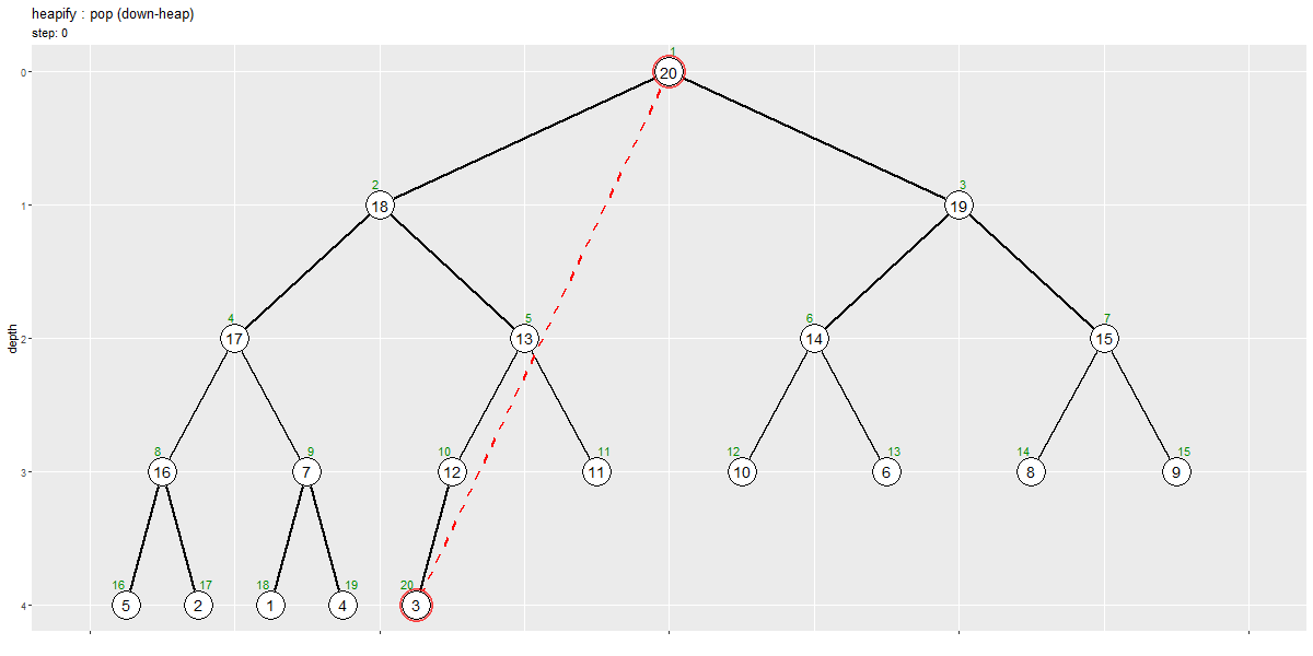
　削除対象または入替対象の頂点を赤色の塗りつぶしで示します。

　ヒープ化されている元の要素数を $N$ とすると、 $1$ 番目(先頭・根)の頂点(要素)を削除して代わりに $N$ 番目(末尾)の要素を挿入します。ヒープ条件を満たさなくなる場合があるので、先頭に挿入した(元末尾の)値と子の値を比較・入替を繰り返します。
　ヒープ条件を満たすまで、挿入値とその子を入れ替えていくことでヒープ化されるのを確認できます。

　この記事では、ヒープ化を実装しました。次の記事では、ヒープソートを実装します。

参考文献

大槻兼資(著), 秋葉拓哉(監修)『問題解決力を鍛える！　アルゴリズムとデータ構造』講談社サイエンティク, 2021年.

おわりに

　面倒臭かった。まず二分木を作図するのが面倒で別記事として書きました。その上、ヒープをベクトルやデータフレームで持つのもややこしい。ただでさえそんな面倒なものを、上手く可視化しようと色とりどりに装飾するんだから輪をかけて面倒でした。
　いえ単に面倒なのはこれまでもあったんでいいんです。そういうことが好きなので、、しかし今回は、面倒ながらも実装した後に、もっと上手い方法があった、もっと上手い見せ方があったと、二度三度と書き直すことになってとても面倒でした。
　分かりながら組んで、組みながら思いついて、試しながら分かって、というスタイルで独学してるのでしょうがないんです。結果満足できるものに仕上がったんでいいんです、はい。面倒だけど。
　あでもヒープ自体は面白かったです。だから深入りしてしまったわけです。

　2023年9月29日は、モーニング娘。の10期メンバー加入12周年です！！！！

　あゆみんがリーダーとして率いるモーニング娘。が観たい！

【次節の内容】

からっぽのしょこ

読んだら書く！書いたら読む！同じ事は二度調べ(たく)ない

【R】10.7：二分ヒープの実装と可視化【『アルゴリズムとデータ構造』のノート】

はじめに

10.7 二分ヒープの実装と可視化

ヒープ化

ヒープ化の実装

ヒープの可視化

ヒープ化の可視化

値の挿入

値の挿入の実装

値の挿入の可視化

ヒープ化の可視化

最大値の削除

最大値の削除の実装

最大値の削除の可視化

参考文献

おわりに