はじめに
『問題解決力を鍛える! アルゴリズムとデータ構造』の学習ノートです。
本に掲載されているコードや図をR言語で再現します。本と一緒に読んでください。
この記事は、12.6節「ソート(4):ヒープソート」の内容です。
ヒープソートのアルゴリズムを確認します。
【前節の内容】
【他の節の内容】
【この節の内容】
12.6 ヒープソートの実装と可視化
二分ヒープ(バイナリヒープ・binary heap)を用いるヒープソート(heap sort)を実装します。また、ソートの推移のアニメーションを作成して、アルゴリズムを確認します。
二分木(バイナリツリー・binary tree)については「ggplot2で二分木を作図したい - からっぽのしょこ」、ヒープについては「【R】10.7:二分ヒープの実装と可視化【『アルゴリズムとデータ構造』のノート】 - からっぽのしょこ」を参照してください。
利用するパッケージを読み込みます。
# 利用パッケージ
library(tidyverse)
library(gganimate)
この記事では、基本的に パッケージ名::関数名() の記法を使っているので、パッケージを読み込む必要はありません。ただし、作図コードについてはパッケージ名を省略しているので、ggplot2 を読み込む必要があります。
また、ネイティブパイプ演算子 |> を使っています。magrittr パッケージのパイプ演算子 %>% に置き換えても処理できますが、その場合は magrittr を読み込む必要があります。
「ソートの可視化」において、gganimate パッケージを利用してアニメーション(gif画像)を作成します。ソートの実装自体には使いません。
ソートの実装
まずは、ヒープソートのアルゴリズムを関数として実装します。
ヒープ化については「【R】10.7:二分ヒープの実装と可視化【『アルゴリズムとデータ構造』のノート】 - からっぽのしょこ」を参照してください。
部分木のヒープ化を実装します。
# 部分木のヒープ化の実装
sub_heapify <- function(vec, i, N) {

  # 左側の子のインデックスを計算
  child_idx <- i * 2

  # 子がなければ終了
  if(child_idx > N) return(vec)

  # 値が大きい方の子のインデックスを設定
  if(child_idx+1 <= N & vec[child_idx+1] > vec[child_idx]) { # (&の左がFALSEだと右が処理されずNAにならないので動く)
    child_idx <- child_idx + 1
  }

  # 子が親以下なら終了
  if(vec[child_idx] <= vec[i]) return(vec)

  # 子と親を入替
  vec[1:N] <- replace(x = vec, list = c(child_idx, i), values = vec[c(i, child_idx)])

  # 子を根としてヒープ化
  vec[1:N] <- sub_heapify(vec, child_idx, N)

  # 数列を出力
  return(vec)
}
数列を vec、入れ替え対象のインデックスを i、数列の要素数を N とします。
i の初期値として部分木の根のインデックスを受け取ります。
i 番目の頂点(要素)の2つの子の内、左側の子のインデックスを child_idx として計算します。頂点 の左側の子
のインデックスは
で求まります。ただし、
のとき、頂点
に子がない(葉である)ことを意味し、入れ替え不要なので、数列をそのまま出力します。
のとき右側の子
が存在するので、2つの子の値が大きい方のインデックスを
childe_idx とします。
子の値 vec[child_idx] と親の値 vec[i] を比較して、子が親以下なら入れ替え不要なので数列をそのまま出力(再帰処理を終了)します。子が親より大きければ値を入れ替えて、childe_idx 番目の頂点を根とする部分木を sub_heapify() でヒープ化します。
sub_heapify() を実行すると内部でさらに(入れ替え対象の頂点が葉になるまで再帰的に) sub_heapify() が実行され、親子の入れ替えが繰り返されて部分木がヒープ化されます。
アルゴリズムの詳しい解説は、本のcode 12.4(前半)などを参照してください。
ヒープソートを実装します。
# ヒープソートの実装
heap_sort <- function(vec) {

  # 数列の要素数を取得
  N <- length(vec)

  # 葉を除くノード番号の最大値を設定
  max_i <- N %/% 2

  # 全体をヒープ化(1個目の最大値を探索)
  for(i in max_i:1) {

    # i番目の頂点を根とする部分木をヒープ化
    vec[1:N] <- sub_heapify(vec, i, N)
  }

  # 全体をソート
  for(i in N:2) { # (後から)

    # ヒープの先頭(N-i+1個目の最大値)をヒープの末尾(前からi番目・後からN-i+1番目の要素と入替
    vec[1:N] <- replace(x = vec, list = c(1, i), values = vec[c(i, 1)])

    # 前からi-1番目までの要素をヒープ化(N-i+2番目の最大値を探索)
    vec[1:(i-1)] <- sub_heapify(vec[1:(i-1)], 1, i-1)
  }

  # 数列を出力
  return(vec)
}
数列を vec、数列の要素数を N とします。
まずは、受け取った数列全体をヒープ化します。
各頂点(要素)を逆順に部分木の根として、sub_heapify() で部分木ごとにヒープ化していきます。ただし、葉(子の無い頂点)はヒープ化不要(ヒープ化済みとみなせる)なので、末尾(N番目)の頂点(要素)の親から処理します。 番目の頂点
の親(葉を除く最後の頂点)
のインデックスは
で求められます。
は、床関数(
floor())で、 以下の最大の整数(小数点以下の切り捨て)を表します。
続いて、ヒープの性質を利用して数列をソートします。
ヒープ化した数列は、先頭(1番目)の要素が最大値になります。つまり、ヒープ化は最大値の探索に対応します。「ヒープの最大値(先頭)」を「ヒープの末尾」と入れ替えて(数列全体における後側に移動して)、残りの数列を再度ヒープ化(次の最大値を探索)します。最大値を削除した際のヒープ化は、一度の処理で行えます。
ヒープ化と最大値の入れ替え(最大値の探索と移動)の操作を交互に繰り返すことで、値が大きい順に探索され、数列の右端(N番目)から順番に並べられます。
最後の要素(要素が1つになった場合)は、ヒープ化と入れ替えは不要です。
アルゴリズムの詳しい解説は、本のcode 12.4(前半)などを参照してください。
実装した関数を試してみます。
要素数を指定して、数列を作成します。
# 要素数を指定
N <- 50

# 数列を生成
a <- sample(x = 1:(2*N), size = N, replace = TRUE)
a
##  [1] 10 57 86 19 49 56 85 69 36 26 53 87 68 64 47 92 26 98 60 79 32 68 75 21 72
## [26] 17 62 24 48 91 95 58 61  3 84 74 46 20 14 38 31 85 53 64 51 60 33 31 21 24
乱数生成関数 sample() などで数値ベクトルを生成します。
ヒープソートにより並べ替えます。
# ソート
heap_sort(a)
##  [1]  3 10 14 17 19 20 21 21 24 24 26 26 31 31 32 33 36 38 46 47 48 49 51 53 53
## [26] 56 57 58 60 60 61 62 64 64 68 68 69 72 74 75 79 84 85 85 86 87 91 92 95 98
目で確認するのはアレなので、組み込み関数のソート結果と比較して確認します。
# 確認
sum(!(heap_sort(a) == sort(a)))
## [1] 0
! で TRUE, FALSE を反転させて sum() で合計することで、一致しない要素数を得られます。結果が 0 であれば全ての要素が一致したことが分かります。
ソートの可視化
次は、ヒープソートのアルゴリズムをグラフで確認します。
親子間のインデックスや座標の計算、バイナリツリーの作成については「ggplot2で二分木を作図したい - からっぽのしょこ」を参照してください。
数列の初期値を作成して、グラフで確認します。
・作図コード(クリックで展開)
要素数を指定して、数列を作成します。
# 要素数を指定
N <- 25

# 数列を生成
a <- rnorm(n = N, mean = 0, sd = 1) |>
  round(digits = 1)
table(a)
## a
## -1.9 -0.8 -0.6 -0.2 -0.1    0  0.1  0.2  0.3  0.5  0.6  0.7  0.8    1  1.8  2.4
##    1    1    1    1    3    2    2    1    2    3    1    3    1    1    1    1
この例では、(負の値を含めるため)正規乱数生成関数 rnorm() で値を生成して、(重複を含めるため)丸め込み関数 round() で小数第一位にしておきます。
数列をデータフレームに格納します。
# 要素数を取得
N <- length(a)

# 数列を格納
tmp_df <- tibble::tibble(
  operation = 0,   # 試行回数
  id        = 1:N, # 元のインデックス
  index     = id,  # 各試行のインデックス
  value     = a,   # 要素
  heap_num  = N,   # ヒープの要素数
  target_flag = FALSE, # 入替対象
  sorted_flag = FALSE  # ソート済み要素
)
tmp_df
## # A tibble: 25 × 7
##    operation    id index value heap_num target_flag sorted_flag
##        <dbl> <int> <int> <dbl>    <int> <lgl>       <lgl>
##  1         0     1     1  -0.1       25 FALSE       FALSE
##  2         0     2     2   0.8       25 FALSE       FALSE
##  3         0     3     3  -0.6       25 FALSE       FALSE
##  4         0     4     4   1         25 FALSE       FALSE
##  5         0     5     5  -0.8       25 FALSE       FALSE
##  6         0     6     6  -0.2       25 FALSE       FALSE
##  7         0     7     7  -1.9       25 FALSE       FALSE
##  8         0     8     8   1.8       25 FALSE       FALSE
##  9         0     9     9   0.7       25 FALSE       FALSE
## 10         0    10    10   0.5       25 FALSE       FALSE
## # ℹ 15 more rows
作図用に、インデックスなどの値とあわせて数列を格納します。数列のみが与えられている場合は、要素数を N とします。
数列を棒グラフで確認します。
# 数列を作図
ggplot() +
  geom_bar(data = tmp_df,
           mapping = aes(x = index, y = value, fill = factor(value)), stat = "identity") +
  theme(panel.grid.minor.x = element_blank()) +
  labs(title = "numerical sequence",
       subtitle = paste0("operation: ", unique(tmp_df[["operation"]])),
       fill = "value",
       x = "index", y = "value")

この要素(バー)を昇順に並べ替えます。
バイナツリーでも確認します。
・作図コード(クリックで展開)
# ノードの座標を作成
d <- 0.6
vertex_df <- tibble::tibble(
  value = a,
  index = 1:length(a),
  depth = floor(log2(index)), # 縦方向のノード位置
  col_idx = index - 2^depth + 1, # 深さごとのノード番号
  coord_x = (col_idx * 2 - 1) * 1/(2^depth * 2), # 横方向のノード位置
  label_offset = dplyr::if_else(
    condition = index%%2 == 0, true = 0.5+d, false = 0.5-d
  ) # ラベル位置を左右にズラす
)

# エッジの座標を作成
edge_df <- dplyr::bind_rows(
  # 子ノードの座標
  vertex_df |>
    dplyr::filter(depth > 0) |> # 根を除去
    dplyr::mutate(
      edge_id   = index,
      node_type = "childe" # (確認用)
    ),
  # 親ノードの座標
  vertex_df |>
    dplyr::filter(depth > 0) |> # 根を除去
    dplyr::mutate(
      edge_id   = index,
      node_type = "parent", # (確認用)
      depth   = depth - 1, # 縦方向のノード位置
      index   = index %/% 2,
      col_idx = index - 2^depth + 1, # 深さごとのノード番号
      coord_x = (col_idx * 2 - 1) * 1/(2^depth * 2) # 横方向のノード位置
    )
) |>
  dplyr::select(!label_offset) |>
  dplyr::arrange(edge_id, depth)

# ツリーの高さを取得
max_h <- floor(log2(N))

# 二分木を作図
d <- 0.1
ggplot() +
  geom_path(data = edge_df,
            mapping = aes(x = coord_x, y = depth, group = edge_id),
            linewidth = 1) + # 辺
  geom_point(data = vertex_df,
             mapping = aes(x = coord_x, y = depth),
             size = 9, shape = "circle filled", fill = "white", stroke = 1) + # 頂点
  geom_text(data = vertex_df,
            mapping = aes(x = coord_x, y = depth, label = value),
            size = 3) + # 値ラベル
  geom_text(data = vertex_df,
            mapping = aes(x = coord_x, y = depth, label = index, hjust = label_offset),
            size = 3, vjust = -2, color = "green4") + # 位置ラベル
  scale_x_continuous(labels = NULL, name = "") +
  scale_y_reverse(breaks = 0:max_h, minor_breaks = FALSE) +
  coord_cartesian(xlim = c(0, 1), ylim = c(max_h+d, -d)) +
  labs(title = "binary tree",
       subtitle = paste0("operation: ", unique(tmp_df[["operation"]])),
       y = "depth")

ヒープ条件(それぞれの分岐で親が子より大きい)を満たしていません。
ヒープ化(数列の入れ替え)時に、値と共にインデックスも入れ替えて出力する関数を定義しておきます。
・作図コード(クリックで展開)
# 部分木のヒープ化の実装
trace_sub_heapify <- function(value, index, i, N) {

  # 値・インデックスを取得
  val_vec <- value
  idx_vec <- index

  # 左側の子のインデックスを計算
  child_idx <- i * 2

  # 子がなければ終了
  if(child_idx > N) {
    lt <- list(value = val_vec, index = idx_vec)
    return(lt)
  }

  # 値が大きい方の子のインデックスを設定
  if(child_idx+1 <= N & val_vec[child_idx+1] > val_vec[child_idx]) { # (&の左がFALSEだと右が処理されずNAにならないので動く)
    child_idx <- child_idx + 1
  }

  # 子が親以下なら終了
  if(val_vec[child_idx] <= val_vec[i]) {
    lt <- list(value = val_vec, index = idx_vec)
    return(lt)
  }

  # 子と親を入替
  val_vec[1:N] <- replace(x = val_vec, list = c(child_idx, i), values = val_vec[c(i, child_idx)])
  idx_vec[1:N] <- replace(x = idx_vec, list = c(child_idx, i), values = idx_vec[c(i, child_idx)])

  # 子を根としてヒープ化
  res_lt <- trace_sub_heapify(val_vec, idx_vec, child_idx, N)
  val_vec[1:N] <- res_lt[["value"]]
  idx_vec[1:N] <- res_lt[["index"]]

  # 数列を出力
  lt <- list(value = val_vec, index = idx_vec)
  return(lt)
}
# ヒープ化の実装
trace_heapify <- function(value, index) {

  # 値・インデックスを取得
  val_vec <- value
  idx_vec <- index
  N       <- length(val_vec)

  # 葉を除くノード番号の最大値を設定
  max_i <- N %/% 2

  # 全体をヒープ化
  for(i in max_i:1) {

    # i番目の頂点を根とする部分木をヒープ化
    res_lt <- trace_sub_heapify(val_vec, idx_vec, i, N)
    val_vec[1:N] <- res_lt[["value"]]
    idx_vec[1:N] <- res_lt[["index"]]
  }

  # 数列を出力
  lt <- list(value = val_vec, index = idx_vec)
  return(lt)
}
数列の値とインデックスを受け取り、sub_heap() と heap_sort() の前半と同様に入れ替えを行い、作図用の値を出力します。
作図用の値として、「数列の値・インデックス」のベクトルをリストに格納して出力します。
数列全体をヒープ化します。
・作図コード(クリックで展開)
# 作図用のオブジェクトを初期化
id_vec   <- 1:N
trace_df <- tmp_df

# 数列をヒープ化
res_lt <- trace_heapify(a, id_vec)
a[1:N]      <- res_lt[["value"]]
id_vec[1:N] <- res_lt[["index"]]

# 数列を格納
tmp_df <- tibble::tibble(
  operation = 1,
  id        = id_vec,
  index     = 1:N,
  value     = a,
  heap_num  = N,
  target_flag = FALSE,
  sorted_flag = FALSE
)
tmp_df
## # A tibble: 25 × 7
##    operation    id index value heap_num target_flag sorted_flag
##        <dbl> <int> <int> <dbl>    <int> <lgl>       <lgl>
##  1         1    14     1   2.4       25 FALSE       FALSE
##  2         1     8     2   1.8       25 FALSE       FALSE
##  3         1    12     3   0.6       25 FALSE       FALSE
##  4         1     4     4   1         25 FALSE       FALSE
##  5         1    10     5   0.5       25 FALSE       FALSE
##  6         1    25     6   0.3       25 FALSE       FALSE
##  7         1    15     7   0         25 FALSE       FALSE
##  8         1     2     8   0.8       25 FALSE       FALSE
##  9         1     9     9   0.7       25 FALSE       FALSE
## 10         1    21    10   0.5       25 FALSE       FALSE
## # ℹ 15 more rows
数列のヒープ化に対応するようにインデックスも入れ替えて、データフレームに格納します。
先ほどのコードで、数列を棒グラフとツリーで確認します。

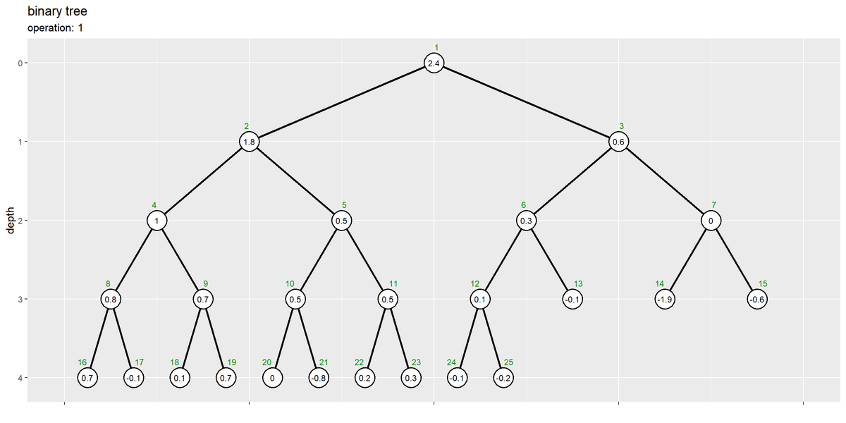
数列全体がヒープ化された状態です。
アルゴリズムに従いソートを行って、作図用のデータを作成します。
・作図コード(クリックで展開)
1試行ずつ入れ替え処理を行い、数列を記録します。
# 数列を記録
trace_df <- dplyr::bind_rows(trace_df, tmp_df)

# 全体をソート
iter <- 1
for(i in N:2) {

  ## 最大値の入替操作

  # N-i+1個目の最大値をヒープの末尾と入替
  a[1:N]      <- replace(x = a, list = c(1, i), values = a[c(i, 1)])
  id_vec[1:N] <- replace(x = id_vec, list = c(1, i), values = id_vec[c(i, 1)])

  # 数列を格納
  tmp_df <- tibble::tibble(
    operation = iter + 1,
    id        = id_vec,
    index     = 1:N,
    value     = a,
    heap_num  = i, # (作図用に入れ替え後もi番目をヒープとしておく)
    target_flag = index %in% c(1, i), # 入替要素:(最大値と末尾)
    sorted_flag = index >= i
  )

  # 数列を記録
  trace_df <- dplyr::bind_rows(trace_df, tmp_df)

  # 途中経過を表示
  #print(paste0("--- operation: ", iter+1, " ---"))
  #print(a)

  ## ヒープ化(最大値の探索)操作

  # 要素が1つならヒープ化不要
  if(i == 2) break

  # i-1番目までの要素をヒープ化(N-i+2個目の最大値を探索)
  res_lt <- trace_sub_heapify(a[1:(i-1)], id_vec[1:(i-1)], i = 1, N = i-1)
  a[1:(i-1)]      <- res_lt[["value"]]
  id_vec[1:(i-1)] <- res_lt[["index"]]

  # 数列を格納
  tmp_df <- tibble::tibble(
    operation = iter + 2,
    id        = id_vec,
    index     = 1:N,
    value     = a,
    heap_num  = i - 1,
    target_flag = FALSE,
    sorted_flag = index >= i
  )

  # 数列を記録
  trace_df <- dplyr::bind_rows(trace_df, tmp_df)

  # 試行回数をカウント
  iter <- iter + 2
}
「ソートの実装」(heap_sort() の後半)のときと同様にして、要素を入れ替えていきます。
数列 a の初期値のインデックス(1 から N の整数)を id_vec としておき、a の要素の入れ替えに対応するように id_vec の要素も入れ替えます。
試行ごとに、数列やインデックスをデータフレームに保存します。
各試行における、ヒープ部分の先頭(最大値)と末尾の要素は target_flag 列を TRUE、ソートされた(ヒープ部分でない)要素は sorted_flag 列を TRUE にします。
初期値のときのコードで、最終結果の数列を棒グラフとツリーで確認します。


数列全体が昇順にソートされた状態です。ヒープ条件は満たしていません。
各試行の数列の棒グラフを切り替えて推移を確認します。
・作図コード(クリックで展開)
重複ラベルの描画用のデータフレームを作成します。
# 重複ラベルを作成
dup_label_df <- trace_df |>
  dplyr::arrange(operation, id) |> # IDの割当用
  dplyr::group_by(operation, value) |> # IDの割当用
  dplyr::mutate(
    dup_id    = dplyr::row_number(id), # 重複IDを割当
    dup_num   = max(dup_id), # 重複の判定用
    dup_label = dplyr::if_else(
      condition = dup_num > 1, true = paste0("(", dup_id, ")"), false = ""
    ) # 重複要素のみラベルを作成
  ) |>
  dplyr::ungroup() |>
  dplyr::arrange(operation, index)
dup_label_df |>
  dplyr::select(!heap_num) # (資料作成用に間引き)
## # A tibble: 1,225 × 9
##    operation    id index value target_flag sorted_flag dup_id dup_num dup_label
##        <dbl> <int> <int> <dbl> <lgl>       <lgl>        <int>   <int> <chr>
##  1         0     1     1  -0.1 FALSE       FALSE            1       3 "(1)"
##  2         0     2     2   0.8 FALSE       FALSE            1       1 ""
##  3         0     3     3  -0.6 FALSE       FALSE            1       1 ""
##  4         0     4     4   1   FALSE       FALSE            1       1 ""
##  5         0     5     5  -0.8 FALSE       FALSE            1       1 ""
##  6         0     6     6  -0.2 FALSE       FALSE            1       1 ""
##  7         0     7     7  -1.9 FALSE       FALSE            1       1 ""
##  8         0     8     8   1.8 FALSE       FALSE            1       1 ""
##  9         0     9     9   0.7 FALSE       FALSE            1       3 "(1)"
## 10         0    10    10   0.5 FALSE       FALSE            1       3 "(1)"
## # ℹ 1,215 more rows
各試行の数列データ trace_df を用いて、重複している値の要素にのみそれぞれ通し番号のラベルを作成します。
最大値と入替対象の描画用のデータフレームを作成します。
# 入替対象の座標を作成
range_swap_df <- trace_df |>
  dplyr::filter(operation%%2 == 1) |> # 入替前のデータを抽出
  dplyr::group_by(operation) |> # 入替対象の抽出用
  dplyr::filter(index %in% c(1, N-0.5*(operation-1))) |> # 入替対象の抽出
  dplyr::ungroup() |>
  dplyr::mutate(
    bar_label = paste0("iter: ", operation+1, ", idx: ", index)
  )
range_swap_df
## # A tibble: 48 × 8
##    operation    id index value heap_num target_flag sorted_flag bar_label
##        <dbl> <int> <int> <dbl>    <dbl> <lgl>       <lgl>       <chr>
##  1         1    14     1   2.4       25 FALSE       FALSE       iter: 2, idx: 1
##  2         1     6    25  -0.2       25 FALSE       FALSE       iter: 2, idx: 25
##  3         3     8     1   1.8       24 FALSE       FALSE       iter: 4, idx: 1
##  4         3     1    24  -0.1       24 FALSE       FALSE       iter: 4, idx: 24
##  5         5     4     1   1         23 FALSE       FALSE       iter: 6, idx: 1
##  6         5    23    23   0.3       23 FALSE       FALSE       iter: 6, idx: 23
##  7         7     2     1   0.8       22 FALSE       FALSE       iter: 8, idx: 1
##  8         7    22    22   0.2       22 FALSE       FALSE       iter: 8, idx: 22
##  9         9    16     1   0.7       21 FALSE       FALSE       iter: 10, idx: 1
## 10         9     5    21  -0.8       21 FALSE       FALSE       iter: 10, idx: …
## # ℹ 38 more rows
各試行における入れ替え前(ヒープ化後)の数列全体(operation 列が奇数)の行を取り出して、ヒープの先頭と末尾(index 列が )の行を取り出します。(
target_flag 列が TRUE なのは入れ替え後のデータです。)
最大値の描画用のデータフレームを作成します。
# ヒープの最大値を作成
upper_df <- trace_df |>
  dplyr::filter(target_flag) |> # 入替時のデータを抽出
  dplyr::group_by(operation) |> # 最大値の抽出用
  dplyr::filter(index != 1) |> # 最大値を抽出
  dplyr::ungroup() |>
  dplyr::mutate(
    operation = operation - 1 # 表示フレームを調整
  )
upper_df
## # A tibble: 24 × 7
##    operation    id index value heap_num target_flag sorted_flag
##        <dbl> <int> <int> <dbl>    <dbl> <lgl>       <lgl>
##  1         1    14    25   2.4       25 TRUE        TRUE
##  2         3     8    24   1.8       24 TRUE        TRUE
##  3         5     4    23   1         23 TRUE        TRUE
##  4         7     2    22   0.8       22 TRUE        TRUE
##  5         9    16    21   0.7       21 TRUE        TRUE
##  6        11     9    20   0.7       20 TRUE        TRUE
##  7        13    19    19   0.7       19 TRUE        TRUE
##  8        15    12    18   0.6       18 TRUE        TRUE
##  9        17    10    17   0.5       17 TRUE        TRUE
## 10        19    21    16   0.5       16 TRUE        TRUE
## # ℹ 14 more rows
入れ替え後(target_flag 列が TRUE)のデータ(行)を取り出して、最大値(index 列が 1 でない)の行を取り出します。
ヒープ化要素の描画用のデータフレームを作成します。
# ヒープ範囲の座標を作成
d <- 0.2
range_heap_df <- tibble::tibble(
  operation = 0:(2*(N-1)),
  left  = 1,
  right = c(NA, N, rep((N-1):2, each = 2), 0),
  x     = 0.5 * (left + right),
  y     = 0.5 * (max(a) + min(c(0, a))),
  w     = right - left + 1,
  h     = max(a) - min(c(0, a)) + d
)
range_heap_df
## # A tibble: 49 × 7
##    operation  left right     x     y     w     h
##        <int> <dbl> <dbl> <dbl> <dbl> <dbl> <dbl>
##  1         0     1    NA  NA    0.25    NA   4.5
##  2         1     1    25  13    0.25    25   4.5
##  3         2     1    24  12.5  0.25    24   4.5
##  4         3     1    24  12.5  0.25    24   4.5
##  5         4     1    23  12    0.25    23   4.5
##  6         5     1    23  12    0.25    23   4.5
##  7         6     1    22  11.5  0.25    22   4.5
##  8         7     1    22  11.5  0.25    22   4.5
##  9         8     1    21  11    0.25    21   4.5
## 10         9     1    21  11    0.25    21   4.5
## # ℹ 39 more rows
ヒープの要素数は、初回時(1回目・operation 列が 1)はN個であり、入替と探索の2回ごとに1個ずつ減っていきます。ただし、初期値(0回目)は0個で、最終試行(2N-1回目)では2個減り0個になります。
各試行におけるヒープ要素(バー)を囲うように座標を作成します。
ソート済み要素の描画用のデータフレームを作成します。
# ソート済み範囲の座標を作成
range_sort_df <- tibble::tibble(
  operation = 0:(2*(N-1)),
  left  = c(NA, N+1, rep(N:3, each = 2), 1),
  right = N,
  x     = 0.5 * (left + right),
  y     = 0.5 * (max(a) + min(c(0, a))),
  w     = right - left + 1,
  h     = max(a) - min(c(0, a)) + d
)
range_sort_df
## # A tibble: 49 × 7
##    operation  left right     x     y     w     h
##        <int> <dbl> <int> <dbl> <dbl> <dbl> <dbl>
##  1         0    NA    25  NA    0.25    NA   4.5
##  2         1    26    25  25.5  0.25     0   4.5
##  3         2    25    25  25    0.25     1   4.5
##  4         3    25    25  25    0.25     1   4.5
##  5         4    24    25  24.5  0.25     2   4.5
##  6         5    24    25  24.5  0.25     2   4.5
##  7         6    23    25  24    0.25     3   4.5
##  8         7    23    25  24    0.25     3   4.5
##  9         8    22    25  23.5  0.25     4   4.5
## 10         9    22    25  23.5  0.25     4   4.5
## # ℹ 39 more rows
ヒープの要素数とは逆に右端から数えて、ソート済み要素数は、初回時(1回目・operation 列が 1)は0個であり、入替と探索の2回ごとに1個ずつ増えていきます。ただし、初期値(0回目)は0個で、最終試行(2N-1回目)では2個増えN個になります。
各試行におけるソート済み要素(バー)を囲うように座標を作成します。
推移のアニメーションを作成します。
# ソートのアニメーションを作図
graph <- ggplot() +
  geom_tile(data = range_heap_df,
            mapping = aes(x = x, y = y, width = w, height = h, color = "heap"),
            fill = "blue", alpha = 0.1, linewidth = 1, linetype = "dashed", na.rm = TRUE) + # ヒープ範囲
  geom_tile(data = range_sort_df,
            mapping = aes(x = x, y = y, width = w, height = h, color = "sort"),
            fill = "orange", alpha = 0.1, linewidth = 1, linetype = "dashed", na.rm = TRUE) + # ソート済み範囲
  geom_bar(data = range_swap_df,
           mapping = aes(x = index, y = value, color = "max", group = bar_label),
           stat = "identity",
           fill = "red", alpha = 0.1, linewidth = 1, linetype = "dashed") + # 入替対象
  geom_bar(data = trace_df,
           mapping = aes(x = index, y = value, fill = factor(value), group = id),
           stat = "identity", show.legend = FALSE) + # 全ての要素
  geom_text(data = trace_df,
            mapping = aes(x = index, y = 0, label = as.character(value), group = id),
            vjust = -0.5, size = 4) + # 要素ラベル
  geom_text(data = dup_label_df,
            mapping = aes(x = index, y = 0, label = dup_label, group = id),
            vjust = 1, size = 3) + # 重複ラベル
  geom_hline(data = upper_df,
             mapping = aes(yintercept = value),
             color = "red", linewidth = 1, linetype = "dotted") + # ヒープの最大値
  gganimate::transition_states(states = operation, transition_length = 9, state_length = 1, wrap = FALSE) + # フレーム遷移
  gganimate::ease_aes("cubic-in-out") + # 遷移の緩急
  scale_color_manual(breaks = c("max", "heap", "sort"),
                     values = c("red", "blue", "orange"),
                     labels = c("swap", "heap", "sorted"),
                     name = "bar") + # (凡例表示用)
  guides(color = guide_legend(override.aes = list(fill = c("red", "blue", "orange")))) + # 凡例の体裁
  theme(panel.grid.minor.x = element_blank()) +
  labs(title = "heap sort",
       subtitle = "operation: {next_state}",
       x = "index", y = "value")

# フレーム数を設定
frame_num <- max(trace_df[["operation"]]) + 1
frame_num <- 2 * N - 1

# 遷移フレーム数を指定
s <- 20

# gif画像を作成
gganimate::animate(
  plot = graph,
  nframes = (frame_num + 2)*s, start_pause = s, end_pause = s, fps = 20,
  width = 900, height = 600,
  renderer = gganimate::gifski_renderer()
)
transition_states() のフレーム制御の引数 states に試行回数列 operation を指定して、これまでと同様に作図します。
animate() の plot 引数にグラフオブジェクト、nframes 引数にフレーム数を指定して、gif画像を作成します。
初期値を含み・要素ごとに最大値の探索と入替の繰り返し・ただし1要素の場合は処理が不要なため、試行回数は です。
transition_states() でアニメーションを作成すると、フレーム間の値を補完して、状態の遷移を描画します。遷移のフレームを s として、試行回数の s 倍の値を nframes 引数に指定します。
ヒープとして扱う要素を青色、ヒープの先頭(最大値)と末尾の要素を赤色、ソート済みの要素をオレンジ色の塗りつぶし枠で示します。また、各試行における最大値を赤色の水平線で示します。
最大値の探索(ヒープ化)と入替(削除)を繰り返すことで、降順に(右端から)ソートされるのを確認できます。青色の枠内のバー(要素)は赤線よりも小さく、オレンジ色の枠内のバーよりも大きいのが分かります。
また、重複要素の順序が入れ替わる(安定性・stable性がない)も確認できます。
ここでの試行回数(operationの値)は、この可視化方法における試行番号(作図処理上の値)であり他の手法と対応していません。
続いて、各試行の数列のバイナツリーを切り替えて推移を確認します。
・作図コード(クリックで展開)
試行ごとの頂点の描画用のデータフレームを作成します。
# 頂点の座標を作成
trace_vertex_df <- trace_df |>
  dplyr::mutate(
    depth   = floor(log2(index)), # 縦方向のノード位置
    col_idx = index - 2^depth + 1,
    coord_x = (col_idx * 2 - 1) * 1/(2^depth * 2), # 横方向のノード位置
  ) |>
  dplyr::arrange(operation, index)
trace_vertex_df |>
  dplyr::select(!heap_num) # (資料作成用に間引き)
## # A tibble: 1,225 × 9
##    operation    id index value target_flag sorted_flag depth col_idx coord_x
##        <dbl> <int> <int> <dbl> <lgl>       <lgl>       <dbl>   <dbl>   <dbl>
##  1         0     1     1  -0.1 FALSE       FALSE           0       1  0.5
##  2         0     2     2   0.8 FALSE       FALSE           1       1  0.25
##  3         0     3     3  -0.6 FALSE       FALSE           1       2  0.75
##  4         0     4     4   1   FALSE       FALSE           2       1  0.125
##  5         0     5     5  -0.8 FALSE       FALSE           2       2  0.375
##  6         0     6     6  -0.2 FALSE       FALSE           2       3  0.625
##  7         0     7     7  -1.9 FALSE       FALSE           2       4  0.875
##  8         0     8     8   1.8 FALSE       FALSE           3       1  0.0625
##  9         0     9     9   0.7 FALSE       FALSE           3       2  0.188
## 10         0    10    10   0.5 FALSE       FALSE           3       3  0.312
## # ℹ 1,215 more rows
各試行の数列データ trace_df を用いて、試行ごとに(step 列でグループ化して)、「ヒープの可視化」のときと同様にして、頂点の座標を計算します。
辺の描画用のデータフレームを作成します。
# 辺の座標を作成
edge_df <- dplyr::bind_rows(
  # 子ノードの座標
  trace_vertex_df |>
    dplyr::filter(operation == 0, depth > 0) |> # 1試行分のデータを抽出・根を除去
    dplyr::mutate(
      edge_id = index
    ),
  # 親ノードの座標
  trace_vertex_df |>
    dplyr::filter(operation == 0, depth > 0) |> # 1試行分のデータを抽出・根を除去
    dplyr::mutate(
      edge_id = index, # 子インデックス
      depth   = depth - 1,
      index   = index %/% 2, # 親インデックス
      col_idx = index - 2^depth + 1,
      coord_x = (col_idx * 2 - 1) * 1/(2^depth * 2)
    )
) |>
  dplyr::select(!operation) |> # フレーム遷移の影響から外す
  dplyr::arrange(edge_id, depth)
edge_df |>
  dplyr::select(!col_idx) # (資料作成用に間引き)
## # A tibble: 48 × 9
##       id index value heap_num target_flag sorted_flag depth coord_x edge_id
##    <int> <dbl> <dbl>    <dbl> <lgl>       <lgl>       <dbl>   <dbl>   <int>
##  1     2     1   0.8       25 FALSE       FALSE           0   0.5         2
##  2     2     2   0.8       25 FALSE       FALSE           1   0.25        2
##  3     3     1  -0.6       25 FALSE       FALSE           0   0.5         3
##  4     3     3  -0.6       25 FALSE       FALSE           1   0.75        3
##  5     4     2   1         25 FALSE       FALSE           1   0.25        4
##  6     4     4   1         25 FALSE       FALSE           2   0.125       4
##  7     5     2  -0.8       25 FALSE       FALSE           1   0.25        5
##  8     5     5  -0.8       25 FALSE       FALSE           2   0.375       5
##  9     6     3  -0.2       25 FALSE       FALSE           1   0.75        6
## 10     6     6  -0.2       25 FALSE       FALSE           2   0.625       6
## # ℹ 38 more rows
1試行分(この例だと初期値)の頂点の座標データを取り出して、「ヒープの可視化」のときと同様にして、辺(始点・終点)の座標を計算します。
インデックスラベルの描画用のデータフレームを作成します。
# インデックスラベルの座標を作成
d <- 0.6
index_df <- trace_vertex_df |>
  dplyr::filter(operation == 0) |> # 1試行分のデータを抽出
  dplyr::mutate(
    offset = dplyr::if_else(
      condition = index%%2 == 0, true = 0.5+d, false = 0.5-d
    ) # ラベル位置を左右にズラす
  ) |>
  dplyr::select(!operation) # フレーム遷移の影響から外す
index_df |>
  dplyr::select(!col_idx) # (資料作成用に間引き)
## # A tibble: 25 × 9
##       id index value heap_num target_flag sorted_flag depth coord_x offset
##    <int> <int> <dbl>    <dbl> <lgl>       <lgl>       <dbl>   <dbl>  <dbl>
##  1     1     1  -0.1       25 FALSE       FALSE           0  0.5      -0.1
##  2     2     2   0.8       25 FALSE       FALSE           1  0.25      1.1
##  3     3     3  -0.6       25 FALSE       FALSE           1  0.75     -0.1
##  4     4     4   1         25 FALSE       FALSE           2  0.125     1.1
##  5     5     5  -0.8       25 FALSE       FALSE           2  0.375    -0.1
##  6     6     6  -0.2       25 FALSE       FALSE           2  0.625     1.1
##  7     7     7  -1.9       25 FALSE       FALSE           2  0.875    -0.1
##  8     8     8   1.8       25 FALSE       FALSE           3  0.0625    1.1
##  9     9     9   0.7       25 FALSE       FALSE           3  0.188    -0.1
## 10    10    10   0.5       25 FALSE       FALSE           3  0.312     1.1
## # ℹ 15 more rows
1試行分の頂点の座標データを取り出して、「ヒープの可視化」のときと同様にして、ラベル位置の調整値を追加します。
重複ラベルの描画用のデータフレームを作成します。
# 重複ラベルを作成
dup_label_df <- trace_vertex_df |>
  dplyr::arrange(operation, id) |> # IDの割当用
  dplyr::group_by(operation, value) |> # IDの割当用
  dplyr::mutate(
    dup_id    = dplyr::row_number(id), # 重複IDを割当
    dup_num   = max(dup_id), # 重複の判定用
    dup_label = dplyr::if_else(
      condition = dup_num > 1, true = paste0("(", dup_id, ")"), false = ""
    ) # 重複要素のみラベルを作成
  ) |>
  dplyr::ungroup() |>
  dplyr::arrange(operation, index)
dup_label_df |>
  dplyr::select(!c(target_flag, sorted_flag, col_idx, coord_x)) # (資料作成用に間引き)
## # A tibble: 1,225 × 9
##    operation    id index value heap_num depth dup_id dup_num dup_label
##        <dbl> <int> <int> <dbl>    <dbl> <dbl>  <int>   <int> <chr>
##  1         0     1     1  -0.1       25     0      1       3 "(1)"
##  2         0     2     2   0.8       25     1      1       1 ""
##  3         0     3     3  -0.6       25     1      1       1 ""
##  4         0     4     4   1         25     2      1       1 ""
##  5         0     5     5  -0.8       25     2      1       1 ""
##  6         0     6     6  -0.2       25     2      1       1 ""
##  7         0     7     7  -1.9       25     2      1       1 ""
##  8         0     8     8   1.8       25     3      1       1 ""
##  9         0     9     9   0.7       25     3      1       3 "(1)"
## 10         0    10    10   0.5       25     3      1       3 "(1)"
## # ℹ 1,215 more rows
「棒グラフによる可視化」のときと同様にして、重複ラベルを作成します。
入れ替え対象・ヒープ化済み・ソート済みの頂点の描画用のデータフレームを作成します。
# 入替対象の頂点の座標を作成
target_vertex_df <- dplyr::bind_rows(
  # 最大値との入替要素の座標
  trace_vertex_df |>
    dplyr::filter(target_flag) |> # 入替要素を抽出
    dplyr::mutate(
      vertex_type = "max"
    ),
  # (ヒープの最大値・末尾を除く)ヒープ化要素の座標
  trace_vertex_df |>
    dplyr::filter(operation > 1, !sorted_flag, !target_flag) |> # ヒープ要素を抽出
    dplyr::mutate(
      vertex_type = "heap"
    ),
  # ソート済み要素の座標
  trace_vertex_df |>
    dplyr::filter(sorted_flag, !target_flag) |> # ソート済み要素を抽出
    dplyr::mutate(
      vertex_type = "sort"
    ),
  # フレーム調整用に最終値を複製
  trace_vertex_df |>
    dplyr::filter(operation == max(operation)) |> # 最終結果を抽出
    dplyr::mutate(
      vertex_type = "sort",
      heap_num    = 0,
      target_flag = FALSE,
      sorted_flag = TRUE,
      operation   = operation + 1 # フレーム調整用
    ),
  tibble::tibble(
    operation = 1
  ) # (フレーム順の謎バグ回避用)
) |>
  dplyr::mutate(
    vertex_label = paste0("iter: ", operation, ", idx: ", index),
    operation = operation - 1 # 表示フレームを調整
  ) |>
  dplyr::arrange(operation, index)
target_vertex_df |>
  dplyr::select(!c(value, heap_num, col_idx, coord_x)) # (資料作成用に間引き)
## # A tibble: 1,201 × 8
##    operation    id index target_flag sorted_flag depth vertex_type vertex_label
##        <dbl> <int> <int> <lgl>       <lgl>       <dbl> <chr>       <chr>
##  1         0    NA    NA NA          NA             NA <NA>        iter: 1, idx…
##  2         1     6     1 TRUE        FALSE           0 max         iter: 2, idx…
##  3         1     8     2 FALSE       FALSE           1 heap        iter: 2, idx…
##  4         1    12     3 FALSE       FALSE           1 heap        iter: 2, idx…
##  5         1     4     4 FALSE       FALSE           2 heap        iter: 2, idx…
##  6         1    10     5 FALSE       FALSE           2 heap        iter: 2, idx…
##  7         1    25     6 FALSE       FALSE           2 heap        iter: 2, idx…
##  8         1    15     7 FALSE       FALSE           2 heap        iter: 2, idx…
##  9         1     2     8 FALSE       FALSE           3 heap        iter: 2, idx…
## 10         1     9     9 FALSE       FALSE           3 heap        iter: 2, idx…
## # ℹ 1,191 more rows
各試行の頂点の座標データ trace_vertex_df から、最大値との入れ替え要素・ヒープ要素・ソート済み要素をそれぞれ取り出して結合します。
入れ替え要素は、target_flag 列が TRUE の行を取り出します。
ヒープ要素は、sorted_flag 列が FALSE の行を取り出します。ただし、初期値と初回時のデータ、各試行のヒープの最大値は除きます。
ソート済み要素は、sorted_flag 列が TRUE の行を取り出します。
1試行早く表示するために、step 列を-1し、最終値(全ての要素がソート済み)のデータを複製します。
入れ替え対象の頂点を結ぶ辺の描画用のデータフレームを作成します。
# 最大値との入替対象の辺の座標を計算
swap_edge_df <- target_vertex_df |>
  dplyr::filter(target_flag) |> # 入替要素を抽出
  dplyr::arrange(operation, index)
swap_edge_df |>
  dplyr::select(!c(value, heap_num, col_idx, coord_x)) # (資料作成用に間引き)
## # A tibble: 48 × 8
##    operation    id index target_flag sorted_flag depth vertex_type vertex_label
##        <dbl> <int> <int> <lgl>       <lgl>       <dbl> <chr>       <chr>
##  1         1     6     1 TRUE        FALSE           0 max         iter: 2, idx…
##  2         1    14    25 TRUE        TRUE            4 max         iter: 2, idx…
##  3         3     1     1 TRUE        FALSE           0 max         iter: 4, idx…
##  4         3     8    24 TRUE        TRUE            4 max         iter: 4, idx…
##  5         5    23     1 TRUE        FALSE           0 max         iter: 6, idx…
##  6         5     4    23 TRUE        TRUE            4 max         iter: 6, idx…
##  7         7    22     1 TRUE        FALSE           0 max         iter: 8, idx…
##  8         7     2    22 TRUE        TRUE            4 max         iter: 8, idx…
##  9         9     5     1 TRUE        FALSE           0 max         iter: 10, id…
## 10         9    16    21 TRUE        TRUE            4 max         iter: 10, id…
## # ℹ 38 more rows
各試行の頂点ごとの属性・座標データ target_vertex_df から、各試行の入れ替え要素(target_flag 列が TRUE)の行を取り出します。(これは試行回数列が欠損していても問題ない理由が分からない。)
ヒープ化済みの頂点を結ぶ辺の描画用のデータフレームを作成します。
# ヒープ対象の辺の座標を計算
heap_edge_df <- dplyr::bind_rows(
  # 親の座標
  target_vertex_df |>
    dplyr::filter(index <= heap_num%/%2) |> # 葉とソート済み要素を除去
    tidyr::uncount(weights = 2, .id = "childe_id") |> # 子の数に複製
    dplyr::mutate(
      vertex_type = "heap",
      childe_id = childe_id - 1, # 行番号を子IDに変換
      edge_id   = index*2+childe_id # 子インデックス
    ) |>
  dplyr::filter(edge_id <= heap_num), # 子がなければ除去
  # 子の座標
  target_vertex_df |>
    dplyr::filter(index > 1, index <= heap_num) |> # 根とソート済み要素を除去
    dplyr::mutate(
      vertex_type = "heap",
      edge_id = index
    ),
  tibble::tibble(
    operation = 0
  ) # (フレーム順の謎バグ回避用)
) |>
  dplyr::mutate(
    edge_label = paste0("iter: ", operation+1, ", idx: ", edge_id)
  ) |>
  dplyr::arrange(operation, edge_id, index)
heap_edge_df |>
  dplyr::select(!c(value, heap_num, depth, col_idx, coord_x, vertex_type, vertex_label)) # (資料作成用に間引き)
## # A tibble: 1,153 × 8
##    operation    id index target_flag sorted_flag childe_id edge_id edge_label
##        <dbl> <int> <int> <lgl>       <lgl>           <dbl>   <dbl> <chr>
##  1         0    NA    NA NA          NA                 NA      NA iter: 1, idx…
##  2         1     6     1 TRUE        FALSE               0       2 iter: 2, idx…
##  3         1     8     2 FALSE       FALSE              NA       2 iter: 2, idx…
##  4         1     6     1 TRUE        FALSE               1       3 iter: 2, idx…
##  5         1    12     3 FALSE       FALSE              NA       3 iter: 2, idx…
##  6         1     8     2 FALSE       FALSE               0       4 iter: 2, idx…
##  7         1     4     4 FALSE       FALSE              NA       4 iter: 2, idx…
##  8         1     8     2 FALSE       FALSE               1       5 iter: 2, idx…
##  9         1    10     5 FALSE       FALSE              NA       5 iter: 2, idx…
## 10         1    12     3 FALSE       FALSE               0       6 iter: 2, idx…
## # ℹ 1,143 more rows
ヒープ要素の親と子のデータをそれぞれ取り出して結合します。sorted_flag 列が FALSE のデータは入れ替え後の最大値を含みません。
親の頂点として「1番目から葉を除いた(末尾の親までの)要素」、子の頂点として「根を除いたヒープの要素数(heap_num 列)番目の要素」取り出します。親のデータは、子の数に対応するように複製します。
推移のアニメーションを作成します。
# ヒープソートのアニメーションを作図
max_h <- floor(log2(N))
d <- 0.1
graph <- ggplot() +
  geom_path(data = edge_df,
            mapping = aes(x = coord_x, y = depth, group = edge_id),
            linewidth = 1) + # 辺
  geom_path(data = heap_edge_df,
            mapping = aes(x = coord_x, y = depth, group = edge_label),
            color = "blue", linewidth = 1, linetype = "dashed", na.rm = TRUE) + # ヒープ対象の辺
  geom_path(data = swap_edge_df,
            mapping = aes(x = coord_x, y = depth, group = operation),
            color = "red", linewidth = 1, linetype = "dashed", na.rm = TRUE) + # 入替対象の辺
  geom_point(data = target_vertex_df,
             mapping = aes(x = coord_x, y = depth, color = vertex_type, group = vertex_label),
             size = 12, alpha = 0.6, na.rm = TRUE) + # 頂点ごとの属性
  geom_point(data = trace_vertex_df,
             mapping = aes(x = coord_x, y = depth, group = id),
             size = 9, shape = "circle filled", fill = "white", stroke = 1) + # 頂点
  geom_text(data = trace_vertex_df,
            mapping = aes(x = coord_x, y = depth, label = as.character(value), group = id),
            size = 3) + # 値ラベル
  geom_text(data = dup_label_df,
            mapping = aes(x = coord_x, y = depth, label = dup_label, group = id),
            size = 3, vjust = 2.6) + # 重複ラベル
  geom_text(data = index_df,
            mapping = aes(x = coord_x, y = depth, label = index, hjust = offset),
            size = 3, vjust = -2, color = "green4") + # インデックスラベル
  gganimate::transition_states(states = operation, transition_length = 9, state_length = 1, wrap = FALSE) + # フレーム遷移
  gganimate::ease_aes("cubic-in-out") + # 遷移の緩急
  scale_x_continuous(labels = NULL) +
  scale_y_reverse(breaks = 0:max_h, minor_breaks = FALSE) +
  scale_color_manual(breaks = c("max", "heap", "sort"),
                     values = c("red", "blue", "orange"),
                     labels = c("swap", "heap", "sorted"),
                     name = "vertex") + # (凡例表示用)
  coord_cartesian(xlim = c(0, 1), ylim = c(max_h+d, -d)) +
  labs(title = "heap sort",
       subtitle = "operation: {next_state}",
       x = "", y = "depth")

# フレーム数を取得
frame_num <- max(trace_df[["operation"]]) + 1

# 遷移フレーム数を指定
s <- 20

# gif画像を作成
gganimate::animate(
  plot = graph,
  nframes = (frame_num + 2)*s, start_pause = s, end_pause = s, fps = 20,
  width = 800, height = 400,
  renderer = gganimate::gifski_renderer()
)
ヒープとして扱う要素を青色、ヒープの先頭(最大値)と末尾の要素を赤色、ソート済みの要素をオレンジ色の塗りつぶしで示します。
最大値の探索(ヒープ化)と入替(削除)を繰り返すことで、降順に(右下から)ソートされるのを確認できます。また、ヒープ化時の入れ替えが、一連の頂点(子孫間)の入れ替えなのが分かります。
この記事では、ヒープソートを実装しました。次の記事では、バケットソートを実装します。
参考文献
- 大槻兼資(著), 秋葉拓哉(監修)『問題解決力を鍛える! アルゴリズムとデータ構造』講談社サイエンティク, 2021年.
おわりに
執筆順的に言うとこの手法が最後でした。バケットソートが面白そうだったので先にやってしまっただけなんですが、これを読みもせずに後回しにして正解でした。それくらい面倒でした。どれくらい面倒臭かったかと言うと、この記事のために別の記事を2つ用意する必要がありました。このアルゴリズムの理解にも繋がるので、ぜひそっちも読んでみてください。
面倒というのはあくまで可視化のためにアレコレする手間の話で、アルゴリズムの実装自体はどれもどっこいどっこいです。
全ての手法で、1要素ずつバーを動かして計算量の違いを比較できる形でアニメーション化したかったのですが、力不足かつ力尽きました。次の機会には、今回扱った手法以外も含めて挑戦したいです。
投稿日に公開された新MVをどうぞ。
褒められたいとは言わないけど正直もう少しアクセス数が伸びてほしーナほしーノ。
【次節の内容】