はじめに

　調べても分からなかったので自分なりにやってみる黒魔術シリーズです。もっといい方法があれば教えてください。

　この記事では、ggplot2パッケージを利用してバイナリツリーのグラフを作成します。

【他の内容】

www.anarchive-beta.com

【目次】

はじめに
ggplot2で二分木を作図したい
参考文献
おわりに

ggplot2で二分木を作図したい

　ggplot2パッケージを利用して、二分木(二進木・バイナリーツリー・binary tree)のグラフを作成する。

　利用するパッケージを読み込む。

# 利用パッケージ
library(tidyverse)

　この記事では、基本的に パッケージ名::関数名() の記法を使っているので、パッケージを読み込む必要はない。ただし、作図コードについてはパッケージ名を省略しているので、ggplot2 を読み込む必要がある。
　また、ネイティブパイプ演算子 |> を使っている。magrittrパッケージのパイプ演算子 %>% に置き換えても処理できるが、その場合は magrittr を読み込む必要がある。

二分木の作成

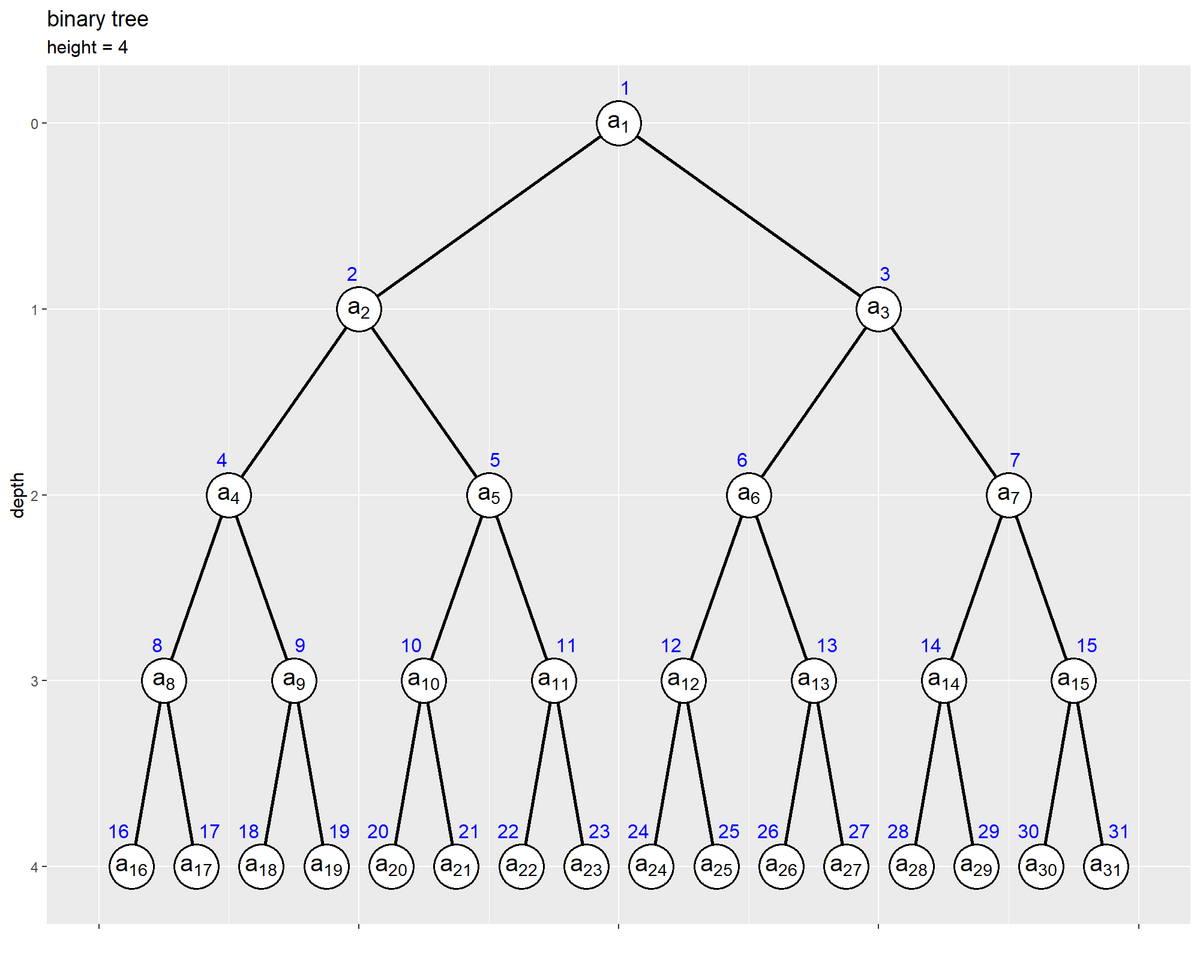
　まずは簡易版として、「上から下」また「左から右」方向に欠損なくノード(要素)が並ぶ二分木のグラフを作成する。
　ただし、最初のノード(要素)のインデックスを1とする(Rが1からなので)。インデックスを0から割り当てる場合は「ggplot2でn分木を作図したい - からっぽのしょこ」を参照のこと。

　ノード数を指定して、値を作成する。

# ノード数を指定
N <- 31

# (簡易的に)値を作成
a <- 1:N
head(a)

## [1] 1 2 3 4 5 6

　ノード(頂点・節)の数を整数 N として、N 個の値を数値(などの)ベクトル a として作成する。a のみが与えられる場合は、a の要素数を N とする。

　ノードの描画用のデータフレームを作成する。

# ラベル位置の調整値を指定
d <- 0.6

# ノードの座標を作成
node_df <- tibble::tibble(
  value = a, 
  index = 1:N, 
  depth = floor(log2(index)), 
  col_idx = index - 2^depth + 1, # 深さごとのノード番号
  coord_x = (col_idx * 2 - 1) * 1/(2^depth * 2), 
  label_offset = dplyr::if_else(
    condition = index%%2 == 0, true = 0.5+d, false = 0.5-d
  ) # ラベル位置を左右にズラす
)
node_df

## # A tibble: 31 × 6
##    value index depth col_idx coord_x label_offset
##    <int> <int> <dbl>   <dbl>   <dbl>        <dbl>
##  1     1     1     0       1  0.5            -0.1
##  2     2     2     1       1  0.25            1.1
##  3     3     3     1       2  0.75           -0.1
##  4     4     4     2       1  0.125           1.1
##  5     5     5     2       2  0.375          -0.1
##  6     6     6     2       3  0.625           1.1
##  7     7     7     2       4  0.875          -0.1
##  8     8     8     3       1  0.0625          1.1
##  9     9     9     3       2  0.188          -0.1
## 10    10    10     3       3  0.312           1.1
## # ℹ 21 more rows

　この例では、根ノードのインデックスを $i = 1$ 、深さを $h = 0$ とする。

　各ノード(要素) $v_i$ の値 $a_i$ とインデックス $i$ をデータフレームに格納して、深さ $h$ を計算する。各ノード(インデックス)の深さは $h = \lfloor \log_2 i \rfloor$ で求まる。 $\lfloor x \rfloor$ は、床関数(floor())で、 $x$ 以下の最大の整数(小数点以下の切り捨て)を表す。
　各深さにおけるノード番号(位置)を $k$ 、左端のノードを $k = 1$ で表すことにする。左から1番目(左端)のノードのインデックスは $i = 2^h$ なので、左からの位置は $k = i - 2^h + 1$ で求まる。
　各分岐をシンメトリーに描画する場合は、深さごとに、ノード数の2倍の個数 $2 \cdot 2^h$ に等間隔 $\frac{1}{2^{h+1}}$ に分割した $2 k - 1$ 番目の位置にノードを配置する。このとき、x軸の範囲は0から1になる。
　ラベル位置の調整用の値を作成する。この例では、インデックスが偶数の場合は左にズラすために0.5以上の値、奇数の場合は右にズラすために0.5以下の値を格納する。

　エッジの描画用のデータフレームを作成する。

# エッジの座標を作成
edge_df <- dplyr::bind_rows(
  # 子ノードの座標
  node_df |> 
    dplyr::filter(depth > 0) |> # 根を除去
    dplyr::mutate(
      edge_id   = index, 
      node_type = "childe" # (確認用)
    ), 
  # 親ノードの座標
  node_df |> 
    dplyr::filter(depth > 0) |> # 根を除去
    dplyr::mutate(
      edge_id   = index, 
      node_type = "parent", # (確認用)
      depth   = depth - 1, 
      index   = index %/% 2, 
      col_idx = index - 2^depth + 1, # 深さごとのノード番号
      coord_x = (col_idx * 2 - 1) * 1/(2^depth * 2)
    )
) |> 
  dplyr::select(!label_offset) |> 
  dplyr::arrange(edge_id, depth)
edge_df

## # A tibble: 60 × 7
##    value index depth col_idx coord_x edge_id node_type
##    <int> <dbl> <dbl>   <dbl>   <dbl>   <int> <chr>    
##  1     2     1     0       1   0.5         2 parent   
##  2     2     2     1       1   0.25        2 childe   
##  3     3     1     0       1   0.5         3 parent   
##  4     3     3     1       2   0.75        3 childe   
##  5     4     2     1       1   0.25        4 parent   
##  6     4     4     2       1   0.125       4 childe   
##  7     5     2     1       1   0.25        5 parent   
##  8     5     5     2       2   0.375       5 childe   
##  9     6     3     1       2   0.75        6 parent   
## 10     6     6     2       3   0.625       6 childe   
## # ℹ 50 more rows

　親子ノードを結ぶエッジ(辺・枝)の描画用に、子ノードのインデックスを $i$ 、親ノードのインデックスを $j$ として、子ノード $v_i$ と親ノード $v_j$ の座標データをそれぞれ作成して行方向に結合する。
　子ノードのデータは、各ノードのデータ node_df から根ノードのデータ(行)を取り除く。
　親ノードのデータは、各ノードのデータから根ノードのデータを取り除いて親ノードのデータを計算する。親ノードの深さは $h_{(\mathrm{parent})} = h_{(\mathrm{childe})} - 1$ 、インデックスは $j = \lfloor \frac{i}{2} \rfloor$ で求まる。座標などは $j$ を用いて先ほどと同様にして計算する。
　元のノードのインデックスをエッジIDとする。

　バイナリツリーを作成する。

# ツリーの高さを取得
max_h <- max(node_df[["depth"]])
max_h <- floor(log2(N))

# 縦方向の余白の調整値を指定
d <- 0.1

# 二分木を作図
ggplot() + 
  geom_path(data = edge_df, 
            mapping = aes(x = coord_x, y = depth, group = edge_id), 
            linewidth = 1) + # エッジ
  geom_point(data = node_df, 
             mapping = aes(x = coord_x, y = depth), 
             size = 12, shape = "circle filled", fill = "white", stroke = 1) + # ノード
  geom_text(data = node_df, 
            mapping = aes(x = coord_x, y = depth, label = value), 
            size = 5) + # 値ラベル
  geom_text(data = node_df, 
            mapping = aes(x = coord_x, y = depth, label = index, hjust = label_offset), 
            size = 4, vjust = -2, color = "blue") + # 位置ラベル
  scale_x_continuous(labels = NULL, name = "") + 
  scale_y_reverse(breaks = 0:max_h, minor_breaks = FALSE) + 
  coord_cartesian(xlim = c(0, 1), ylim = c(max_h+d, -d)) + 
  labs(title = "binary tree", 
       subtitle = paste0("height = ", max_h), 
       y = "depth")

　エッジとして geom_path() で線分を描画する。線分間が繋がらないように、group 引数にエッジIDを指定する。
　ノードとして geom_point() で点を描画する。枠線と枠内を色分けする場合は、shape 引数に "*** filled" の形状を指定する。
　ラベルを geom_text() でテキストを描画する。ノードやエッジと重ならないように表示する場合は、hjust, vjust 引数に値を指定する。この例では、インデックスが偶数なら左、奇数なら右にズラしている。
　深さ(y軸の値)が大きくなるほど下になるように、scale_y_reverse() でy軸を反転する。

　上の方法では、親子ノードの座標データを同じ列に持つデータフレームを作成して、geom_path() でエッジを描画した。次の方法では、親子ノードの座標データを別の列として持つデータフレームを作成して、geom_segment() でエッジを描画する。

　エッジの描画用のデータフレームを作成する。

# エッジの座標を作成
edge_df <- dplyr::bind_cols(
  # 子ノードの座標
  node_df |> 
    dplyr::filter(depth > 0) |> # 根を除去
    dplyr::select(!label_offset), 
  # 親ノードの座標
  node_df |> 
    dplyr::filter(depth > 0) |> # 根を除去
    dplyr::mutate(
      parent_depth   = depth - 1, 
      parent_index   = index %/% 2, 
      parent_col_idx = parent_index - 2^parent_depth + 1, # 深さごとのノード番号
      parent_coord_x = (parent_col_idx * 2 - 1) * 1/(2^parent_depth * 2)
    ) |> 
    dplyr::select(parent_index, parent_depth, parent_coord_x)
)
edge_df

## # A tibble: 30 × 8
##    value index depth col_idx coord_x parent_index parent_depth parent_coord_x
##    <int> <int> <dbl>   <dbl>   <dbl>        <dbl>        <dbl>          <dbl>
##  1     2     2     1       1  0.25              1            0          0.5  
##  2     3     3     1       2  0.75              1            0          0.5  
##  3     4     4     2       1  0.125             2            1          0.25 
##  4     5     5     2       2  0.375             2            1          0.25 
##  5     6     6     2       3  0.625             3            1          0.75 
##  6     7     7     2       4  0.875             3            1          0.75 
##  7     8     8     3       1  0.0625            4            2          0.125
##  8     9     9     3       2  0.188             4            2          0.125
##  9    10    10     3       3  0.312             5            2          0.375
## 10    11    11     3       4  0.438             5            2          0.375
## # ℹ 20 more rows

　各ノードのデータと親ノードの座標データをそれぞれ作成して列方向に結合(別の列として追加)する。別の列にするために列名を変更して、先ほどと同様にして計算する。

　バイナリツリーを作成する。

# ツリーの高さを取得
max_h <- max(node_df[["depth"]])

# 縦方向の余白の調整値を指定
d <- 0.1

# 二分木を作図
ggplot() + 
  geom_segment(data = edge_df, 
               mapping = aes(x = coord_x, y = depth, xend = parent_coord_x, yend = parent_depth), 
               linewidth = 1) + # エッジ
  geom_point(data = node_df, 
             mapping = aes(x = coord_x, y = depth), 
             size = 12, shape = "circle filled", fill = "white", stroke = 1) + # ノード
  geom_text(data = node_df, 
            mapping = aes(x = coord_x, y = depth, label = paste("a[", index, "]")), parse = TRUE, 
            size = 5) + # 要素ラベル
  geom_text(data = node_df, 
            mapping = aes(x = coord_x, y = depth, label = index, hjust = label_offset), 
            size = 4, vjust = -2, color = "blue") + # 位置ラベル
  scale_x_continuous(labels = NULL, name = "") + 
  scale_y_reverse(breaks = 0:max_h, minor_breaks = FALSE) + 
  coord_cartesian(xlim = c(0, 1), ylim = c(max_h+d, -d)) + 
  labs(title = "binary tree", 
       subtitle = paste0("height = ", max_h), 
       y = "depth")

　geom_segment() でエッジを描画する。始点の座標の引数 x, y に各ノードに関する値、終点の座標の引数 xend, yend に親ノードに関する値を指定する(始点と終点を入れ替えても作図できる)。

　どちらの方法でもグラフ自体には影響しない。ただしこちらは(同じ図を作っても面白くないので)、ノードごとに値ラベルではなく要素ラベルを表示した。

部分木インデックスの計算

　次は、二分木の剪定のために、部分木のインデックスを作成する処理を関数として実装する。

　(手打ちで全てのインデックスを指定するのは嫌なので、)部分木の根ノードのインデックスを指定すると、部分木の全てのインデックスを返す関数を作成しておく。

# 部分木インデックスの定義
subtree <- function(root_index, max_index) {
  
  # 部分木の根インデックスを取得
  parent_idx <- root_index[root_index <= N] |> 
    sort()
  
  # インデックスの最大値を取得
  N <- max_index
  
  # 親ごとに処理
  childe_idx <- NULL
  for(i in parent_idx) {
    
    # 兄弟インデックスを作成
    sibling_idx <- c(2*i, 2*i+1)
    
    # 子インデックスを格納
    childe_idx <- c(childe_idx, sibling_idx[sibling_idx <= N]) # 最大位置を超えたら除去
  }
  
  # 子がなければ再帰処理を終了
  if(length(childe_idx) == 0) return(parent_idx)
  
  # 子孫インデックスを作成
  descendant_idx <- subtree(childe_idx, N)
  
  # 部分木インデックスを格納
  subtree_idx <- c(parent_idx, descendant_idx) |> 
    sort()
  
  # 子孫インデックスを出力
  return(subtree_idx)
}

　親ノードのインデックス $i$ を入力して、子ノードのインデックス $2 i, 2 i + 1$ を格納していく処理を再帰的に行う。ただし、最大インデックス $N$ を超える場合は含めない。

部分木の作成

　二分木の部分木のグラフを作成する。

　ノード数と部分木の根を指定して、部分木を作成する。

# ノード数を指定
N <- 63

# 部分木の根を指定
sub_root_idx <- c(3, 4, 22)

# 部分木のインデックスを作成
sub_node_idx <- subtree(sub_root_idx, N)
sub_node_idx

##  [1]  3  4  6  7  8  9 12 13 14 15 16 17 18 19 22 24 25 26 27 28 29 30 31 32 33
## [26] 34 35 36 37 38 39 44 45 48 49 50 51 52 53 54 55 56 57 58 59 60 61 62 63

　ノードの数(インデックスの最大値)を整数 N として指定する。
　部分木の根ノードのインデックスを整数(複数の場合は整数ベクトル) sub_root_idx として指定して、subtree() で部分木のノードのインデックスを作成して sub_node_idx とする。

　ノードの値から部分木に含まれないノードの値を削除する。

# 値を作成
a <- sample(x = 1:N, size = N, replace = TRUE)

# 部分木以外のノードを剪定
a[!1:N %in% sub_node_idx] <- NA
a

##  [1] NA NA 34 35 NA 43  8 35 19 NA NA  2 10 12 36 29 21 49  4 NA NA 32 NA 19 18
## [26]  4 55 52  1 37 52 53 37 17 27  1 11 41 44 NA NA NA NA  1  3 NA NA 24  4 63
## [51] 24  1 52  4 63 23  4 47 60 32 60 50  8

　N 個の値 a の内、sub_node_idx に含まれない要素を欠損値 NA に置き換える(代入する)。全てのインデックスと値を残すインデックスを %in% 演算子で比較して、! で TRUE, FALSE を反転することで置換できる。

　ノードの描画用のデータフレームを作成する。

# ノードの座標を作成
d <- 0.5
node_df <- tibble::tibble(
  value   = a, 
  node_id = 1:N, 
  index   = dplyr::if_else(
    condition = !is.na(value), true = node_id, false = NA_real_
  ), 
  depth   = floor(log2(index)), 
  col_idx = index - 2^depth + 1, # 深さごとのノード番号
  coord_x = (col_idx * 2 - 1) * 1/(2^depth * 2), 
  label_offset = dplyr::if_else(
    condition = index%%2 == 0, true = 0.5+d, false = 0.5-d
  ) # ラベル位置を左右にズラす
)
node_df

## # A tibble: 63 × 7
##    value node_id index depth col_idx coord_x label_offset
##    <int>   <int> <dbl> <dbl>   <dbl>   <dbl>        <dbl>
##  1    NA       1    NA    NA      NA NA                NA
##  2    NA       2    NA    NA      NA NA                NA
##  3    34       3     3     1       2  0.75              0
##  4    35       4     4     2       1  0.125             1
##  5    NA       5    NA    NA      NA NA                NA
##  6    43       6     6     2       3  0.625             1
##  7     8       7     7     2       4  0.875             0
##  8    35       8     8     3       1  0.0625            1
##  9    19       9     9     3       2  0.188             0
## 10    NA      10    NA    NA      NA NA                NA
## # ℹ 53 more rows

　「二分木の作成」のときと同様に処理する。ただし、ノードのID(通し番号)を node_id 列、値(要素)の欠損に応じて欠損させたIDを index 列とする。
　値やインデックスが欠損値なので、座標データ(深さやx軸座標)の計算結果も欠損値になり、描画されない。

　エッジの描画用のデータフレームを作成する。

# エッジの座標を作成
edge_df <- dplyr::bind_rows(
  # 子ノードの座標
  node_df |> 
    dplyr::filter(depth > 0, !index %in% sub_root_idx) |> # 根を除去
    dplyr::mutate(
      edge_id   = index, 
      node_type = "childe" # (確認用)
    ), 
  # 親ノードの座標
  node_df |> 
    dplyr::filter(depth > 0, !index %in% sub_root_idx) |> # 根を除去
    dplyr::mutate(
      edge_id   = index, 
      node_type = "parent", # (確認用)
      depth   = depth - 1, 
      index   = index %/% 2, 
      col_idx = index - 2^depth + 1, # 深さごとのノード番号
      coord_x = (col_idx * 2 - 1) * 1/(2^depth * 2)
    )
) |> 
  dplyr::select(!label_offset) |> 
  dplyr::arrange(edge_id, depth)
edge_df

## # A tibble: 92 × 8
##    value node_id index depth col_idx coord_x edge_id node_type
##    <int>   <int> <dbl> <dbl>   <dbl>   <dbl>   <dbl> <chr>    
##  1    43       6     3     1       2  0.75         6 parent   
##  2    43       6     6     2       3  0.625        6 childe   
##  3     8       7     3     1       2  0.75         7 parent   
##  4     8       7     7     2       4  0.875        7 childe   
##  5    35       8     4     2       1  0.125        8 parent   
##  6    35       8     8     3       1  0.0625       8 childe   
##  7    19       9     4     2       1  0.125        9 parent   
##  8    19       9     9     3       2  0.188        9 childe   
##  9     2      12     6     2       3  0.625       12 parent   
## 10     2      12    12     3       5  0.562       12 childe   
## # ℹ 82 more rows

　「二分木の作成」のときと同様に処理する。ただし、部分木の根ノードとその親ノードを結ぶエッジが描画されてしまうのを避けるため、部分木の根ノードの行も取り除く。根の除去の際に、欠損ノードのデータ(行)も除去される。

　部分木のバイナリツリーを作成する。

# ツリーの高さを取得
max_h <- floor(log2(N))

# 二分木の部分木を作図
d <- 0.1
ggplot() + 
  geom_path(data = edge_df, 
            mapping = aes(x = coord_x, y = depth, group = edge_id), 
            linewidth = 1) + # エッジ
  geom_point(data = node_df, 
             mapping = aes(x = coord_x, y = depth), 
             size = 10, shape = "circle filled", fill = "white", stroke = 1, na.rm = TRUE) + # ノード
  geom_text(data = node_df, 
            mapping = aes(x = coord_x, y = depth, label = value), 
            size = 4, na.rm = TRUE) + # 値ラベル
  geom_text(data = node_df, 
            mapping = aes(x = coord_x, y = depth, label = index, hjust = label_offset), 
            size = 3, vjust = -2, color = "blue", na.rm = TRUE) + # 位置ラベル
  scale_x_continuous(labels = NULL, name = "") + 
  scale_y_reverse(breaks = 0:max_h, minor_breaks = FALSE) + 
  coord_cartesian(xlim = c(0, 1), ylim = c(max_h+d, -d)) + 
  labs(title = "binary tree", 
       subtitle = "subtree", 
       y = "depth")

　「二分木の作成」のときと同様に処理する。欠損値が含まれるレイヤに na.rm = TRUE を追加すると、警告文が表示されなくなる。元のコードでもグラフ自体には影響しない。

　N個のノードを持つ二分木から、指定した部分木のツリーが得られた。

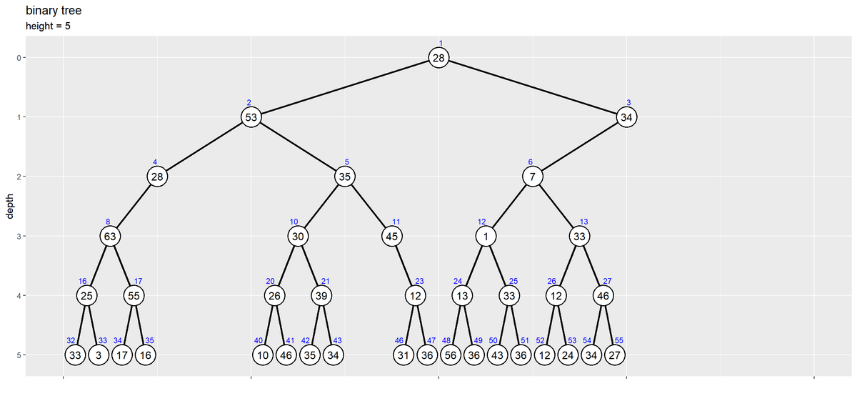
欠損の作成

　続いて、二分木の一部のノード(部分木)を取り除いたグラフを作成する。

　ノード数と削除する部分木の根を指定して、部分木を作成する。

# ノード数を指定
N <- 63

# (削除する)部分木の根を指定
sub_root_idx <- c(7, 9, 22)

# (削除する)部分木のインデックスを作成
del_node_idx <- subtree(sub_root_idx, N)
del_node_idx

##  [1]  7  9 14 15 18 19 22 28 29 30 31 36 37 38 39 44 45 56 57 58 59 60 61 62 63

　「部分木の作成」のときと同様にして、削除する部分木のノードのインデックスを作成して del_node_idx とする。
部分木を含まないノードの値を作成する。

　ノードの値から部分木に含まれるノードの値を削除する。

# 値を作成
a <- sample(x = 1:N, size = N, replace = TRUE)

# 部分木のノードを剪定
a[del_node_idx] <- NA
a

##  [1] 28 53 34 28 35  7 NA 63 NA 30 45  1 33 NA NA 25 55 NA NA 26 39 NA 12 13 33
## [26] 12 46 NA NA NA NA 33  3 17 16 NA NA NA NA 10 46 35 34 NA NA 31 36 56 36 43
## [51] 36 12 24 34 27 NA NA NA NA NA NA NA NA

　N 個の値 a の内、del_node_idx に含まれる要素を欠損値 NA に置き換える(代入する)。

　ノードの描画用のデータフレームを作成する。

# ノードの座標を作成
d <- 0.5
node_df <- tibble::tibble(
  value   = a, 
  node_id = 1:N, 
  index   = dplyr::if_else(
    condition = !is.na(value), true = node_id, false = NA_real_
  ), 
  depth   = floor(log2(index)), 
  col_idx = index - 2^depth + 1, # 深さごとのノード番号
  coord_x = (col_idx * 2 - 1) * 1/(2^depth * 2), 
  label_offset = dplyr::if_else(
    condition = index%%2 == 0, true = 0.5+d, false = 0.5-d
  ) # ラベル位置を左右にズラす
)
node_df

## # A tibble: 63 × 7
##    value node_id index depth col_idx coord_x label_offset
##    <int>   <int> <dbl> <dbl>   <dbl>   <dbl>        <dbl>
##  1    28       1     1     0       1  0.5               0
##  2    53       2     2     1       1  0.25              1
##  3    34       3     3     1       2  0.75              0
##  4    28       4     4     2       1  0.125             1
##  5    35       5     5     2       2  0.375             0
##  6     7       6     6     2       3  0.625             1
##  7    NA       7    NA    NA      NA NA                NA
##  8    63       8     8     3       1  0.0625            1
##  9    NA       9    NA    NA      NA NA                NA
## 10    30      10    10     3       3  0.312             1
## # ℹ 53 more rows

　「部分木の作成」のときのコードで処理する。

　エッジの描画用のデータフレームを作成する。

# エッジの座標を作成
edge_df <- dplyr::bind_rows(
  # 子ノードの座標
  node_df |> 
    dplyr::filter(depth > 0) |> # 根を除去
    dplyr::mutate(
      edge_id   = index, 
      node_type = "childe" # (確認用)
    ), 
  # 親ノードの座標
  node_df |> 
    dplyr::filter(depth > 0) |> # 根を除去
    dplyr::mutate(
      edge_id   = index, 
      node_type = "parent", # (確認用)
      depth   = depth - 1, 
      index   = index %/% 2, 
      col_idx = index - 2^depth + 1, # 深さごとのノード番号
      coord_x = (col_idx * 2 - 1) * 1/(2^depth * 2)
    )
) |> 
  dplyr::select(!label_offset) |> 
  dplyr::arrange(edge_id, depth)
edge_df

## # A tibble: 74 × 8
##    value node_id index depth col_idx coord_x edge_id node_type
##    <int>   <int> <dbl> <dbl>   <dbl>   <dbl>   <dbl> <chr>    
##  1    53       2     1     0       1   0.5         2 parent   
##  2    53       2     2     1       1   0.25        2 childe   
##  3    34       3     1     0       1   0.5         3 parent   
##  4    34       3     3     1       2   0.75        3 childe   
##  5    28       4     2     1       1   0.25        4 parent   
##  6    28       4     4     2       1   0.125       4 childe   
##  7    35       5     2     1       1   0.25        5 parent   
##  8    35       5     5     2       2   0.375       5 childe   
##  9     7       6     3     1       2   0.75        6 parent   
## 10     7       6     6     2       3   0.625       6 childe   
## # ℹ 64 more rows

　「二分木の作成」のときのコードで処理する。

　バイナリツリーを作成する。

# ツリーの高さを取得
max_h <- max(node_df[["depth"]], na.rm = TRUE)

# 二分木を作図
d <- 0.1
ggplot() + 
  geom_path(data = edge_df, 
            mapping = aes(x = coord_x, y = depth, group = edge_id), 
            linewidth = 1) + # エッジ
  geom_point(data = node_df, 
             mapping = aes(x = coord_x, y = depth), 
             size = 10, shape = "circle filled", fill = "white", stroke = 1, na.rm = TRUE) + # ノード
  geom_text(data = node_df, 
            mapping = aes(x = coord_x, y = depth, label = value), 
            size = 4, na.rm = TRUE) + # 値ラベル
  geom_text(data = node_df, 
            mapping = aes(x = coord_x, y = depth, label = index, hjust = label_offset), 
            size = 3, vjust = -2, color = "blue", na.rm = TRUE) + # 位置ラベル
  scale_x_continuous(labels = NULL, name = "") + 
  scale_y_reverse(breaks = 0:max_h, minor_breaks = FALSE) + 
  coord_cartesian(xlim = c(0, 1), ylim = c(max_h+d, -d)) + 
  labs(title = "binary tree", 
       subtitle = paste0("height = ", max_h), 
       y = "depth")

　これまでと同様にして処理する。

　N個のノードを持つ二分木から、指定した(「部分木の作成」における)部分木のノードが欠損したツリーが得られた。

　最後に、値に応じてノードを削除してみる。この例では、根ノードの値未満のノードとその子孫ノードを削除したツリーを作成する。

　ノード数を指定して、値を作成する。

# ノード数を指定
N <- 63

# 値を作成
max_v <- 100
a <- sample(x = 1:max_v, size = N, replace = TRUE)
a

##  [1] 40 72 47 67 20 59 99 89 44 61 20 82 72 51 93 71 61 43 56  4 67 70 13 76 85
## [26] 25 29 29 90 72 24 89 39 69 30 79 96 50  4 62 60 30 22 96 72 80 15 71 15 22
## [51] 26 85 57 71 16 74 64 60 25 77 39 46 72

　(最大値を指定しているが深い意味はない。)

　削除するノードを作成する。

# (削除する)部分木の根を指定
sub_root_idx <- which(x = a < a[1])
sub_root_idx

##  [1]  5 11 20 23 26 27 28 31 33 35 39 42 43 47 49 50 51 55 59 61

　which() を使って条件を満たすインデックスを作成して、削除する根ノードのインデックスとして用いる。

　ノードの値から部分木に含まれるノードの値を削除する。

# (削除する)部分木のインデックスを作成
del_node_idx <- subtree(sub_root_idx, N)

# 部分木のノードを剪定
a[del_node_idx] <- NA
a

##  [1] 40 72 47 67 NA 59 99 89 44 NA NA 82 72 51 93 71 61 43 56 NA NA NA NA 76 85
## [26] NA NA NA 90 72 NA 89 NA 69 NA 79 96 50 NA NA NA NA NA NA NA NA NA 71 NA NA
## [51] NA NA NA NA NA NA NA 60 NA 77 NA NA NA

　先ほどのコードで、バイナリツリーを作成する。

　根の値以上のノードのみが残るツリーが得られた(元のツリーの内、根の値以上のノードの全てが残っているわけではない)。

　この記事では、インデックスが1からのニ分木のグラフを作成した。次の記事では、インデックスが0からで指定した数に分岐するツリーを作成する。

参考文献

大槻兼資(著), 秋葉拓哉(監修)『問題解決力を鍛える！　アルゴリズムとデータ構造』講談社サイエンティク, 2021年.

おわりに

　ヒープソートのために必要だったので書きました。
　それなりに見る図ですし気楽にやるつもりだったのですが、調べてもやり方が見当たらず我流でやることになりました。思いの外面倒でした。だからなかったのか。
　読むだけでも面倒だと思いますが、元が面倒なので仕様がないんです。

　2023年9月14日は、モーニング娘。の結成26周年です！

　ちなみに私は2017年の夏頃からのファンです。これからもよろしくお願いします。

【次の内容】

からっぽのしょこ

読んだら書く！書いたら読む！同じ事は二度調べ(たく)ない

【R】二分木を作図したい【ggplot2】

はじめに

ggplot2で二分木を作図したい

二分木の作成

部分木インデックスの計算

部分木の作成

欠損の作成

参考文献

おわりに