はじめに
調べても分からなかったので自分なりにやってみる黒魔術シリーズです。もっといい方法があれば教えてください。
この記事では、球面上の2点をいい感じに繋ぐ曲線のグラフを作成します。
【前の内容】
【目次】
球面上の2点を結ぶ円弧を作図したい
Matplotlibライブラリを利用して、3次元空間における球面(spherical surface)上の2点を結ぶ良い感じの曲線を作成したい。また、その円弧(circular arc)の半径を調整して、2つの3次元ベクトルのなす角(angle between two vectors)を示したい。
利用するライブラリを読み込みます。
# 利用ライブラリ
import numpy as np
import matplotlib.pyplot as plt
from matplotlib.animation import FuncAnimation
なす角の描画
まずは、完成図(やりたいこと)を確認する。
2つの3次元ベクトルのなす角を円弧(角マーク)で示すグラフを作成する。
なす角については「【Python】3.4:ベクトルとx軸のなす角の可視化【『スタンフォード線形代数入門』のノート】 - からっぽのしょこ」を参照のこと。
3次元ベクトルを作成して、なす角を計算する。
# 3次元ベクトルを指定
a = np.array([1.0, 1.0, 1.0])
b = np.array([-2.0, -0.5, 1.0])

# ベクトルa,bのなす角を計算
cos_theta = np.dot(a, b) / np.linalg.norm(a) / np.linalg.norm(b)
theta = np.arccos(cos_theta)
print(theta) # 0からπの値
print(theta / np.pi) # 0から1の値
1.9583930134500773
0.623375857214425
2つのベクトルを
a, bとして値を指定する。Pythonではインデックスが0から割り当てられるので、は
a[0]に対応することに注意する。
のなす角
は、次の式で計算できる。
はラジアン(弧度法における角度)であり、
の値(度数法による角度
に対応)をとる。ただし、
または
が0ベクトルだと0除算になるため定義できない(計算結果が
nan になる)。
コサイン関数の逆関数(逆コサイン関数)
は
np.arccos()、内積は
np.dot()、ユークリッドノルムは
np.linalg.norm()で計算できる。
角マークと角ラベルの座標を計算するための係数を作成する。
# 角マーク用のラジアンを作成
t = np.linspace(start=0.0, stop=0.5*np.pi, num=100)
print(t[:5])
print(t.shape)

# ラジアンを複製
T = np.stack([t, t, t], axis=1)
print(T[:5])
print(T.shape)

# 角マーク用の係数を作成
Beta1 = np.cos(T)
Beta2 = np.sin(T)

# 角ラベル用のラジアンを作成
t = 0.25 * np.pi

# 角ラベル用の係数を作成
beta1 = np.cos(t)
beta2 = np.sin(t)
print(beta1)
print(beta2)
[0.         0.01586663 0.03173326 0.04759989 0.06346652]
(100,)
[[0.         0.         0.        ]
 [0.01586663 0.01586663 0.01586663]
 [0.03173326 0.03173326 0.03173326]
 [0.04759989 0.04759989 0.04759989]
 [0.06346652 0.06346652 0.06346652]]
(100, 3)
0.7071067811865476
0.7071067811865476
の範囲のラジアン(
に対応)を
tとして、3列分を結合した配列をTとする。
Tを用いて、線形結合に使う係数を計算して
Beta1, Beta2とする。
角ラベルは角マークの中点に配置することにする。
そこで、中点のラジアンを
tとして、を計算して
beta1, beta2とする。
角マークと角ラベルの座標を計算する。
# 角マークのサイズ(なす角からの半径)を指定
r = 0.3

# ベクトルa,b間を結ぶ曲線の座標を計算(ベクトルa,bを線形結合)
X = Beta1 * a/np.linalg.norm(a) + Beta2 * b/np.linalg.norm(b)

# 角マークの座標を計算(サイズを調整)
X *= r / np.linalg.norm(X, axis=1, keepdims=True)
print(X[:5])
print(X.shape)
print(np.linalg.norm(X[:5], axis=1))

# 角ラベルの表示位置(なす角からのノルム)を指定
r = 0.5

# ベクトルa,b間を結ぶ曲線の中点の座標を計算(ベクトルa,bを線形結合)
x = beta1 * a/np.linalg.norm(a) + beta2 * b/np.linalg.norm(b)

# 角ラベルの座標を計算(表示位置を調整)
x *= r / np.linalg.norm(x)
print(x)
print(x.shape)
print(np.linalg.norm(x))
[[0.17320508 0.17320508 0.17320508]
 [0.1700513  0.17318617 0.17632103]
 [0.1668212  0.1731285  0.1794358 ]
 [0.16351323 0.17303067 0.18254811]
 [0.16012584 0.17289119 0.18565654]]
(100, 3)
[0.3 0.3 0.3 0.3 0.3]
[-0.13247569  0.16099114  0.45445797]
(3,)
0.5
を正規化し線形結合したベクトル
を計算して、さらに
を正規化し正の実数
を掛けたベクトルを
とする。
ベクトルをそのベクトルのノルム
で割るとノルムが1になる
。この計算をベクトルの正規化と呼ぶ。
さらに、定数を掛けるとノルムが
の絶対値になる
。
曲線用の係数Beta1, Beta2を用いて求めた座標(2次元配列)をX、ラベル用の係数beta1, beta2を用いて求めた座標(1次元配列)をxとする。Xの各行が1つの点に対応する。
ベクトルとなす角のグラフを作成する。
# グラフサイズ用の値を設定
x_min = np.floor(np.min([0.0, a[0], b[0]])) - 1.0
x_max =  np.ceil(np.max([0.0, a[0], b[0]])) + 1.0
y_min = np.floor(np.min([0.0, a[1], b[1]])) - 1.0
y_max =  np.ceil(np.max([0.0, a[1], b[1]])) + 1.0
z_min = np.floor(np.min([0.0, a[2], b[2]])) - 1.0
z_max =  np.ceil(np.max([0.0, a[2], b[2]])) + 1.0

# 矢のサイズを指定
l = 0.2

# なす角を作図
fig, ax = plt.subplots(figsize=(8, 8), facecolor='white',
                       subplot_kw={'projection': '3d'})
ax.quiver(0, 0, 0, *a,
          color='red', arrow_length_ratio=l/np.linalg.norm(a),
          label='$a=('+', '.join(map(str, a))+')$') # ベクトルa
ax.quiver(0, 0, 0, *b,
          color='blue', arrow_length_ratio=l/np.linalg.norm(b),
          label='$b=('+', '.join(map(str, b.round(2)))+')$') # ベクトルb
ax.plot(*X.T,
        color='black', linewidth=1, zorder=10) # 角マーク
ax.text(*x,
        s='$\\theta$', size=15, ha='center', va='center', zorder=15) # 角ラベル
ax.quiver([0, a[0], b[0]],
          [0, a[1], b[1]],
          [0, a[2], b[2]],
          [0, 0, 0],
          [0, 0, 0],
          [z_min, z_min-a[2], z_min-b[2]],
          color=['gray', 'red', 'blue'],
          arrow_length_ratio=0, linestyle=':') # 座標用の補助線
ax.set_xlim(left=x_min, right=x_max)
ax.set_ylim(bottom=y_min, top=y_max)
ax.set_zlim(bottom=z_min, top=z_max)
ax.set_xlabel('$x_1$')
ax.set_ylabel('$x_2$')
ax.set_zlabel('$x_3$')
ax.set_title('$\\theta=' + str((theta/np.pi).round(2)) + '\pi, ' +
             '\\theta^{\circ}=' + str((theta/np.pi*180.0).round(1)) + '^{\circ}$', loc='left')
fig.suptitle('$\\theta = \\arccos(\\frac{a \cdot b}{\|a\| \|b\|})$', fontsize=20)
ax.legend()
ax.set_aspect('equal')
#ax.view_init(elev=90, azim=270) # xy面
#ax.view_init(elev=0, azim=270) # xz面
#ax.view_init(elev=0, azim=0) # yz面
plt.show()

axes.quiver()の第1・2・3引数に始点の座標、第4・5・6引数にベクトルの移動量を指定する。
各配列の形状に応じて、配列の前に*を付けてアンパック(展開)して座標などを指定している。原点を始点とする。
グラフを回転させて確認する。
・作図コード(クリックで展開)
# フレーム数を指定
frame_num = 60

# 水平方向の角度として利用する値を作成
h_n = np.linspace(start=0.0, stop=360.0, num=frame_num+1)[:frame_num]

# グラフオブジェクトを初期化
fig, ax = plt.subplots(figsize=(8, 8), facecolor='white',
                       subplot_kw={'projection': '3d'})
fig.suptitle('$\\theta = \\arccos(\\frac{a \cdot b}{\|a\| \|b\|})$', fontsize=20)

# 作図処理を関数として定義
def update(i):

    # 前フレームのグラフを初期化
    plt.cla()

    # i番目の角度を取得
    h = h_n[i]

    # なす角を作図
    ax.quiver(0, 0, 0, *a,
              color='red', arrow_length_ratio=l/np.linalg.norm(a),
              label='$a=('+', '.join(map(str, a))+')$') # ベクトルa
    ax.quiver(0, 0, 0, *b,
              color='blue', arrow_length_ratio=l/np.linalg.norm(b),
              label='$b=('+', '.join(map(str, b.round(2)))+')$') # ベクトルb
    ax.plot(*X.T,
            color='black', linewidth=1, zorder=10) # 角マーク
    ax.text(*x,
            s='$\\theta$', size=15, ha='center', va='center', zorder=15) # 角ラベル
    ax.quiver([0, a[0], b[0]],
              [0, a[1], b[1]],
              [0, a[2], b[2]],
              [0, 0, 0],
              [0, 0, 0],
              [z_min, z_min-a[2], z_min-b[2]],
              color=['gray', 'red', 'blue'],
              arrow_length_ratio=0, linestyle=':') # 座標用の補助線
    ax.set_xlim(left=x_min, right=x_max)
    ax.set_ylim(bottom=y_min, top=y_max)
    ax.set_zlim(bottom=z_min, top=z_max)
    ax.set_xlabel('$x_1$')
    ax.set_ylabel('$x_2$')
    ax.set_zlabel('$x_3$')
    ax.set_title('$\\theta=' + str((theta/np.pi).round(2)) + '\pi, ' +
                 '\\theta^{\circ}=' + str((theta/np.pi*180.0).round(1)) + '^{\circ}$', loc='left')
    ax.legend()
    ax.set_aspect('equal')
    ax.view_init(elev=30, azim=h) # 表示角度

# gif画像を作成
ani = FuncAnimation(fig=fig, func=update, frames=frame_num, interval=100)

# gif画像を保存
ani.save(filename='angle360_3d.gif')
作図処理をupdate()として定義して、FuncAnimation()でgif画像を作成する。作成したグラフオブジェクトのsave()メソッドでgifファイルとして書き出す。

ベクトルの値を変化させたアニメーションを作成する。
・作図コード(クリックで展開)
# フレーム数を指定
frame_num = 60

# 固定するベクトルを指定
a = np.array([1.0, 1.0, 1.0])

# 変化するベクトル用のラジアンを作成
t_n = np.linspace(start=0.0, stop=2.0*np.pi, num=frame_num+1)[:frame_num]
u_n = np.linspace(start=2.0/3.0*np.pi, stop=5.0/3.0*np.pi, num=frame_num+1)[:frame_num]

# 変化するベクトルのノルムを指定
d = 2.0

# 変化するベクトルを作成
b_n = np.array(
    [d * np.sin(t_n)*np.cos(u_n), d * np.sin(t_n)*np.sin(u_n), d * np.cos(t_n)]
).T

# 矢のサイズを指定
l = 0.2

# グラフサイズ用の値を設定
axis_size = d
z_min = -axis_size

# グラフオブジェクトを初期化
fig, ax = plt.subplots(figsize=(8, 8), facecolor='white',
                       subplot_kw={'projection': '3d'})
fig.suptitle('$\\theta = \\arccos(\\frac{a \cdot b}{\|a\| \|b\|})$', fontsize=20)

# 作図処理を関数として定義
def update(i):

    # 前フレームのグラフを初期化
    plt.cla()

    # i番目のベクトルを取得
    b = b_n[i]

    # ベクトルa,bのなす角を計算
    theta = np.arccos(np.dot(a, b) / np.linalg.norm(a) / np.linalg.norm(b))

    # 角マークの座標を計算
    r = 0.3
    X = Beta1 * a/np.linalg.norm(a) + Beta2 * b/np.linalg.norm(b) # 2点間の曲線
    X *= r / np.linalg.norm(X, axis=1, keepdims=True) # サイズ調整

    # 角ラベルの座標を計算
    r = 0.5
    x = beta1 * a/np.linalg.norm(a) + beta2 * b/np.linalg.norm(b) # 2点間の中点
    x *= r / np.linalg.norm(x) # サイズ調整

    # なす角を作図
    ax.quiver(0, 0, 0, *a,
              color='red', arrow_length_ratio=l/np.linalg.norm(a),
              label='$a=('+', '.join(map(str, a))+')$') # ベクトルa
    ax.quiver(0, 0, 0, *b,
              color='blue', arrow_length_ratio=l/np.linalg.norm(b),
              label='$b=('+', '.join(map(str, b.round(2)))+')$') # ベクトルb
    ax.plot(*X.T,
            color='black', linewidth=1, zorder=10) # 角マーク
    ax.text(*x,
            s='$\\theta$', size=15, ha='center', va='center', zorder=15) # 角ラベル
    ax.quiver([0, a[0], b[0]],
              [0, a[1], b[1]],
              [0, a[2], b[2]],
              [0, 0, 0],
              [0, 0, 0],
              [z_min, z_min-a[2], z_min-b[2]],
              color=['gray', 'red', 'blue'],
              arrow_length_ratio=0, linestyle=':') # 座標用の補助線
    ax.set_xlim(left=-axis_size, right=axis_size)
    ax.set_ylim(bottom=-axis_size, top=axis_size)
    ax.set_zlim(bottom=-axis_size, top=axis_size)
    ax.set_xlabel('$x_1$')
    ax.set_ylabel('$x_2$')
    ax.set_zlabel('$x_3$')
    ax.set_title('$\\theta=' + str((theta/np.pi).round(2)) + '\pi, ' +
                 '\\theta^{\circ}=' + str((theta/np.pi*180.0).round(1)) + '^{\circ}$', loc='left')
    ax.legend(loc='upper left')
    ax.set_aspect('equal')

# gif画像を作成
ani = FuncAnimation(fig=fig, func=update, frames=frame_num, interval=100)

# gif画像を保存
ani.save(filename='angle_3d.gif')
以上で、なす角を示すグラフを作成できた。次からは、(どの説明が分かりやすいのか分からないので)3つの方法でこの処理(計算)を確認する。
円弧の描画
2つの3次元ベクトルを繋ぐ円弧(角マーク)の座標計算とノルム操作をグラフで確認する。
3次元ベクトルを作成する。
# 3次元ベクトルを指定
a = np.array([1.0, 1.0, 1.0])
b = np.array([-1.0, -1.0, 1.0])
2つのベクトルを
a, bとして値を指定する。
ベクトルのグラフを作成する。
# グラフサイズ用の値を設定
x_min = np.floor(np.min([0.0, a[0], b[0]])) - 1.0
x_max =  np.ceil(np.max([0.0, a[0], b[0]])) + 1.0
y_min = np.floor(np.min([0.0, a[1], b[1]])) - 1.0
y_max =  np.ceil(np.max([0.0, a[1], b[1]])) + 1.0
z_min = np.floor(np.min([0.0, a[2], b[2]])) - 1.0
z_max =  np.ceil(np.max([0.0, a[2], b[2]])) + 1.0

# 矢のサイズを指定
l = 0.2

# ベクトルを作図
fig, ax = plt.subplots(figsize=(8, 8), facecolor='white',
                       subplot_kw={'projection': '3d'})
ax.scatter(0, 0, 0,
           color='orange', s=50, label='$O=(0, 0, 0)$') # 原点
ax.quiver(0, 0, 0, *a,
          color='red', arrow_length_ratio=l/np.linalg.norm(a),
           label='$a=('+', '.join(map(str, a))+')$') # ベクトルa
ax.quiver(0, 0, 0, *b,
          color='blue', arrow_length_ratio=l/np.linalg.norm(b),
           label='$b=('+', '.join(map(str, b))+')$') # ベクトルb
ax.quiver([0, a[0], b[0]],
          [0, a[1], b[1]],
          [0, a[2], b[2]],
          [0, 0, 0],
          [0, 0, 0],
          [z_min, z_min-a[2], z_min-b[2]],
          color=['orange', 'red', 'blue'],
          arrow_length_ratio=0, linestyle=':') # 座標用の補助線
ax.set_xticks(ticks=np.arange(x_min, x_max+0.1, 0.5))
ax.set_yticks(ticks=np.arange(y_min, y_max+0.1, 0.5))
ax.set_zticks(ticks=np.arange(z_min, z_max+0.1, 0.5))
ax.set_zlim(bottom=z_min, top=z_max)
ax.set_xlabel('x')
ax.set_ylabel('y')
ax.set_zlabel('z')
ax.set_title('$\|a\|=' + str(np.linalg.norm(a).round(2)) + ', ' +
             '\|b\|=' + str(np.linalg.norm(b).round(2)) + '$', loc='left')
fig.suptitle('vectors', fontsize=20)
ax.legend()
ax.set_aspect('equal')
plt.show()

axes.quiver()の第1・2・3引数に始点の座標、第4・5・6引数にベクトルの移動量を指定する。
各配列の形状に応じて、配列の前に*を付けてアンパック(展開)して座標などを指定している。原点を始点とする。
原点からのノルムを指定して、ベクトル上の点(ノルムが
のベクトル)
を計算する。
# 円弧の半径を指定
r = 0.5

# ベクトルのノルムを調整
tilde_a = r * a / np.linalg.norm(a)
tilde_b = r * b / np.linalg.norm(b)
print(tilde_a)
print(np.linalg.norm(tilde_a))
print(tilde_b)
print(np.linalg.norm(tilde_b))
[0.28867513 0.28867513 0.28867513]
0.5
[-0.28867513 -0.28867513  0.28867513]
0.5
をそれぞれ正規化し正の実数
を掛けて、ノルムを
に変更したベクトル
を
tilde_a, tilde_bとする。
ノルムの操作については「なす角の描画」を参照のこと。
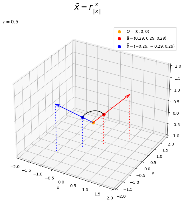
ベクトル上の点
のグラフを作成する。
# ベクトル上の点を作図
fig, ax = plt.subplots(figsize=(8, 8), facecolor='white',
                       subplot_kw={'projection': '3d'})
ax.scatter(0, 0, 0,
           color='orange', s=50, label='$O=(0, 0, 0)$') # 原点
ax.scatter(*tilde_a,
           color='red', s=50,
           label='$\\tilde{a}=('+', '.join(map(str, tilde_a.round(2)))+')$') # ベクトルa上の点
ax.scatter(*tilde_b,
           color='blue', s=50,
           label='$\\tilde{b}=('+', '.join(map(str, tilde_b.round(2)))+')$') # ベクトルb上の点
ax.quiver(0, 0, 0, *a,
          color='red', arrow_length_ratio=l/np.linalg.norm(a)) # ベクトルa
ax.quiver(0, 0, 0, *b,
          color='blue', arrow_length_ratio=l/np.linalg.norm(b)) # ベクトルb
ax.quiver([0, a[0], b[0], tilde_a[0], tilde_b[0]],
          [0, a[1], b[1], tilde_a[1], tilde_b[1]],
          [0, a[2], b[2], tilde_a[2], tilde_b[2]],
          [0, 0, 0, 0, 0],
          [0, 0, 0, 0, 0],
          [z_min, z_min-a[2], z_min-b[2], z_min-tilde_a[2], z_min-tilde_b[2]],
          color=['orange', 'red', 'blue', 'red', 'blue'],
          arrow_length_ratio=0, linestyle=':') # 座標用の補助線
ax.set_xticks(ticks=np.arange(x_min, x_max+0.1, 0.5))
ax.set_yticks(ticks=np.arange(y_min, y_max+0.1, 0.5))
ax.set_zticks(ticks=np.arange(z_min, z_max+0.1, 0.5))
ax.set_zlim(bottom=z_min, top=z_max)
ax.set_xlabel('x')
ax.set_ylabel('y')
ax.set_zlabel('z')
ax.set_title('$r=' + str(r) + ', ' +
             '\|\\tilde{a}\|=' + str(np.linalg.norm(tilde_a).round(2)) + ', ' +
             '\|\\tilde{b}\|=' + str(np.linalg.norm(tilde_b).round(2)) + '$', loc='left')
fig.suptitle('$\\tilde{a} = r \\frac{a}{\|a\|}, ' +
             '\\tilde{b} = r \\frac{b}{\|b\|}$', fontsize=20)
ax.legend()
ax.set_aspect('equal')
plt.show()

点がそれぞれ、ベクトル
と平行な直線上で、原点からのノルムが
の点になるのを確認できる。
ベクトルを線形結合して、点
を結ぶ曲線を計算する。
# 曲線用のラジアンを作成
t = np.linspace(start=0.0, stop=0.5*np.pi, num=100)
print(t[:5])

# 曲線用の係数を作成
beta1 = np.cos(t)
beta2 = np.sin(t)
print(beta1[:5])
print(beta2[:5])

# 2点間の曲線の座標を計算
x = beta1 * tilde_a[0] + beta2 * tilde_b[0]
y = beta1 * tilde_a[1] + beta2 * tilde_b[1]
z = beta1 * tilde_a[2] + beta2 * tilde_b[2]
print(x[:5])
print(y[:5])
print(z[:5])
[0.         0.01586663 0.03173326 0.04759989 0.06346652]
[1.         0.99987413 0.99949654 0.99886734 0.99798668]
[0.         0.01586596 0.03172793 0.04758192 0.06342392]
[0.28867513 0.28405869 0.27937073 0.27461245 0.26978503]
[0.28867513 0.28405869 0.27937073 0.27461245 0.26978503]
[0.28867513 0.29321891 0.29768886 0.30208388 0.30640285]
、
であるのを利用して、線形結合の係数を
とする。
の範囲のラジアンを用いると、係数は
の値をとる。
ベクトルを線形結合したベクトルを
とする。
をそれぞれ計算して
x, y, zとする。x, y, zの各インデックスが1つの点に対応する。
を結ぶ曲線のグラフを作成する。
# 2点間の曲線を作図
fig, ax = plt.subplots(figsize=(8, 8), facecolor='white',
                       subplot_kw={'projection': '3d'})
ax.scatter(0, 0, 0,
           color='orange', s=50, label='$O=(0, 0, 0)$') # 原点
ax.scatter(*tilde_a,
           color='red', s=50,
           label='$\\tilde{a}=('+', '.join(map(str, tilde_a.round(2)))+')$') # ベクトルa上の点
ax.scatter(*tilde_b,
           color='blue', s=50,
           label='$\\tilde{b}=('+', '.join(map(str, tilde_b.round(2)))+')$') # ベクトルb上の点
ax.quiver(0, 0, 0, *a,
          color='red', arrow_length_ratio=l/np.linalg.norm(a)) # ベクトルa
ax.quiver(0, 0, 0, *b,
          color='blue', arrow_length_ratio=l/np.linalg.norm(b)) # ベクトルb
ax.plot(x, y, z,
        color='black', zorder=10) # 2点間の曲線
ax.quiver([0, a[0], b[0], tilde_a[0], tilde_b[0]],
          [0, a[1], b[1], tilde_a[1], tilde_b[1]],
          [0, a[2], b[2], tilde_a[2], tilde_b[2]],
          [0, 0, 0, 0, 0],
          [0, 0, 0, 0, 0],
          [z_min, z_min-a[2], z_min-b[2], z_min-tilde_a[2], z_min-tilde_b[2]],
          color=['orange', 'red', 'blue', 'red', 'blue'],
          arrow_length_ratio=0, linestyle=':') # 座標用の補助線
ax.set_xticks(ticks=np.arange(x_min, x_max+0.1, 0.5))
ax.set_yticks(ticks=np.arange(y_min, y_max+0.1, 0.5))
ax.set_zticks(ticks=np.arange(z_min, z_max+0.1, 0.5))
ax.set_zlim(bottom=z_min, top=z_max)
ax.set_xlabel('x')
ax.set_ylabel('y')
ax.set_zlabel('z')
ax.set_title('$0 \leq t \leq \\frac{\pi}{2}$', loc='left')
fig.suptitle('$x = \cos t\ \\tilde{a} + \sin t\ \\tilde{b}$', fontsize=20)
ax.legend()
ax.set_aspect('equal')
plt.show()

係数を変化させた線形結合の点
を繋いだ曲線が、点
を結ぶ曲線になるのを確認できる。
曲線のノルムをに変更する。
# 曲線の座標を結合
xyz = np.stack([x, y, z], axis=1)
print(xyz[:5])
print(xyz.shape)

# 点ごとにノルムを計算
norm_xyz = np.linalg.norm(xyz, axis=1)
print(norm_xyz[:5])
print(norm_xyz.shape)

# 曲線のノルムを調整
tilde_x = r * x / norm_xyz
tilde_y = r * y / norm_xyz
tilde_z = r * z / norm_xyz
print(tilde_x[:5])
print(tilde_y[:5])
print(tilde_z[:5])
print(np.linalg.norm(np.stack([tilde_x, tilde_y, tilde_z], axis=1), axis=1)[:5])
[[0.28867513 0.28867513 0.28867513]
 [0.28405869 0.28405869 0.29321891]
 [0.27937073 0.27937073 0.29768886]
 [0.27461245 0.27461245 0.30208388]
 [0.26978503 0.26978503 0.30640285]]
(100, 3)
[0.5        0.49734898 0.49468644 0.4920149  0.48933693]
(100,)
[0.28867513 0.28557281 0.28237153 0.27906924 0.27566388]
[0.28867513 0.28557281 0.28237153 0.27906924 0.27566388]
[0.28867513 0.29478185 0.30088642 0.30698651 0.31307963]
[0.5 0.5 0.5 0.5 0.5]
を正規化し正の実数
を掛けて、ノルムを
に変更したベクトルを
とする。
をそれぞれ計算して
tilde_x, tilde_y, tilde_zとする。tilde_x, tilde_y, tilde_zの各インデックスが1つの点に対応する。
を結ぶ円弧(原点からのノルムが
の曲線)のグラフを作成する。
# 2点間の円弧を作図
fig, ax = plt.subplots(figsize=(8, 8), facecolor='white',
                       subplot_kw={'projection': '3d'})
ax.scatter(0, 0, 0,
           color='orange', s=50, label='$O=(0, 0, 0)$') # 原点
ax.scatter(*tilde_a,
           color='red', s=50,
           label='$\\tilde{a}=('+', '.join(map(str, tilde_a.round(2)))+')$') # ベクトルa上の点
ax.scatter(*tilde_b,
           color='blue', s=50,
           label='$\\tilde{b}=('+', '.join(map(str, tilde_b.round(2)))+')$') # ベクトルb上の点
ax.quiver(0, 0, 0, *a,
          color='red', arrow_length_ratio=l/np.linalg.norm(a)) # ベクトルa
ax.quiver(0, 0, 0, *b,
          color='blue', arrow_length_ratio=l/np.linalg.norm(b)) # ベクトルb
ax.plot(tilde_x, tilde_y, tilde_z,
        color='black', zorder=10) # 2点間の円弧
ax.quiver([0, a[0], b[0], tilde_a[0], tilde_b[0]],
          [0, a[1], b[1], tilde_a[1], tilde_b[1]],
          [0, a[2], b[2], tilde_a[2], tilde_b[2]],
          [0, 0, 0, 0, 0],
          [0, 0, 0, 0, 0],
          [z_min, z_min-a[2], z_min-b[2], z_min-tilde_a[2], z_min-tilde_b[2]],
          color=['orange', 'red', 'blue', 'red', 'blue'],
          arrow_length_ratio=0, linestyle=':') # 座標用の補助線
ax.set_xticks(ticks=np.arange(x_min, x_max+0.1, 0.5))
ax.set_yticks(ticks=np.arange(y_min, y_max+0.1, 0.5))
ax.set_zticks(ticks=np.arange(z_min, z_max+0.1, 0.5))
ax.set_zlim(bottom=z_min, top=z_max)
ax.set_xlabel('x')
ax.set_ylabel('y')
ax.set_zlabel('z')
ax.set_title('$r=' + str(r) + '$', loc='left')
fig.suptitle('$\\tilde{x} = r \\frac{x}{\|x\|}$', fontsize=20)
ax.legend()
ax.set_aspect('equal')
#ax.view_init(elev=90, azim=270) # xy面
#ax.view_init(elev=0, azim=270) # xz面
#ax.view_init(elev=0, azim=0) # yz面
plt.show()
ベクトルを結ぶいい感じの曲線が得られた。
グラフを回転させて確認する。
・作図コード(クリックで展開)
# フレーム数を指定
frame_num = 60

# 水平方向の角度として利用する値を作成
h_n = np.linspace(start=0.0, stop=360.0, num=frame_num+1)[:frame_num]

# グラフオブジェクトを初期化
fig, ax = plt.subplots(figsize=(8, 8), facecolor='white',
                       subplot_kw={'projection': '3d'})
fig.suptitle('circular arc', fontsize=20)

# 作図処理を関数として定義
def update(i):

    # 前フレームのグラフを初期化
    plt.cla()

    # i番目の角度を取得
    h = h_n[i]

    # 2点間の円弧を作図
    ax.scatter(0, 0, 0,
               color='orange', s=50, label='$O=(0, 0, 0)$') # 原点
    ax.scatter(*tilde_a,
               color='red', s=50,
               label='$\\tilde{a}=('+', '.join(map(str, tilde_a.round(2)))+')$') # ベクトルa上の点
    ax.scatter(*tilde_b,
               color='blue', s=50,
               label='$\\tilde{b}=('+', '.join(map(str, tilde_b.round(2)))+')$') # ベクトルb上の点
    ax.quiver(0, 0, 0, *a,
              color='red', arrow_length_ratio=l/np.linalg.norm(a)) # ベクトルa
    ax.quiver(0, 0, 0, *b,
              color='blue', arrow_length_ratio=l/np.linalg.norm(b)) # ベクトルb
    ax.plot(x, y, z,
            color='purple', zorder=10) # 2点間の曲線
    ax.plot(tilde_x, tilde_y, tilde_z,
            color='black', zorder=10) # 2点間の円弧
    ax.quiver([0, a[0], b[0], tilde_a[0], tilde_b[0]],
              [0, a[1], b[1], tilde_a[1], tilde_b[1]],
              [0, a[2], b[2], tilde_a[2], tilde_b[2]],
              [0, 0, 0, 0, 0],
              [0, 0, 0, 0, 0],
              [z_min, z_min-a[2], z_min-b[2], z_min-tilde_a[2], z_min-tilde_b[2]],
              color=['orange', 'red', 'blue', 'red', 'blue'],
              arrow_length_ratio=0, linestyle=':') # 座標用の補助線
    ax.set_xticks(ticks=np.arange(x_min, x_max+0.1, 0.5))
    ax.set_yticks(ticks=np.arange(y_min, y_max+0.1, 0.5))
    ax.set_zticks(ticks=np.arange(z_min, z_max+0.1, 0.5))
    ax.set_zlim(bottom=z_min, top=z_max)
    ax.set_xlabel('x')
    ax.set_ylabel('y')
    ax.set_zlabel('z')
    ax.set_title('$r=' + str(r) + '$', loc='left')
    ax.legend()
    ax.set_aspect('equal')
    ax.view_init(elev=30, azim=h) # 表示角度

# gif画像を作成
ani = FuncAnimation(fig=fig, func=update, frames=frame_num, interval=100)

# gif画像を保存
ani.save(filename='arc360_3d.gif')
正規化したベクトルの線形結合
を紫色の曲線、ノルムを調整した円弧
を黒色の曲線で描画する。
ベクトルの値を変化させたアニメーションを作成する。
・作図コード(クリックで展開)
# フレーム数を指定
frame_num = 60

# 円弧の半径を指定
r = 0.5

# 固定するベクトルを指定
a = np.array([1.0, 1.0, 1.0])
tilde_a = r * a / np.linalg.norm(a) # ノルムを調整

# 変化するベクトル用のラジアンを作成
t_n = np.linspace(start=-1.0*np.pi, stop=1.0*np.pi, num=frame_num+1)[:frame_num]
u_n = np.linspace(start=2.0/3.0*np.pi, stop=5.0/3.0*np.pi, num=frame_num+1)[:frame_num]

# 変化するベクトルのサイズを指定
d = 2.0

# 変化するベクトルを作成
b_n = np.array(
    [d * np.sin(t_n)*np.cos(u_n), d * np.sin(t_n)*np.sin(u_n), d * np.cos(t_n)]
).T

# 矢のサイズを指定
l = 0.2

# グラフサイズ用の値を設定
axis_size = np.ceil(d)
z_min = -axis_size

# グラフオブジェクトを初期化
fig, ax = plt.subplots(figsize=(8, 8), facecolor='white',
                       subplot_kw={'projection': '3d'})
fig.suptitle('circular arc', fontsize=20)

# 作図処理を関数として定義
def update(i):

    # 前フレームのグラフを初期化
    plt.cla()

    # i番目のベクトルを取得
    b = b_n[i]
    tilde_b = r * b / np.linalg.norm(b) # ノルムを調整

    # ベクトルa,bのなす角を計算
    theta = np.arccos(np.dot(a, b) / np.linalg.norm(a) / np.linalg.norm(b))

    # 2点間の曲線の座標を計算
    x = beta1 * tilde_a[0] + beta2 * tilde_b[0]
    y = beta1 * tilde_a[1] + beta2 * tilde_b[1]
    z = beta1 * tilde_a[2] + beta2 * tilde_b[2]

    # 点ごとにノルムを計算
    norm_xyz = np.linalg.norm(np.stack([x, y, z], axis=1), axis=1)

    # 曲線のノルムを調整
    tilde_x = r * x / norm_xyz
    tilde_y = r * y / norm_xyz
    tilde_z = r * z / norm_xyz

    # 2点間の円弧を作図
    ax.scatter(0, 0, 0,
               color='orange', s=50, label='$O=(0, 0, 0)$') # 原点
    ax.scatter(*tilde_a,
               color='red', s=50,
               label='$\\tilde{a}=('+', '.join(map(str, tilde_a.round(2)))+')$') # ベクトルa上の点
    ax.scatter(*tilde_b,
               color='blue', s=50,
               label='$\\tilde{b}=('+', '.join(map(str, tilde_b.round(2)))+')$') # ベクトルb上の点
    ax.quiver(0, 0, 0, *a,
              color='red', arrow_length_ratio=l/np.linalg.norm(a)) # ベクトルa
    ax.quiver(0, 0, 0, *b,
              color='blue', arrow_length_ratio=l/np.linalg.norm(b)) # ベクトルb
    ax.quiver(0, 0, z_min, a[0], a[1], 0,
              color='red', linestyle='--', arrow_length_ratio=l/np.linalg.norm(a)) # 底面上のベクトルa
    ax.quiver(0, 0, z_min, b[0], b[1], 0,
              color='blue', linestyle='--', arrow_length_ratio=l/np.linalg.norm(b)) # 底面上のベクトルb
    ax.plot(x, y, z,
            color='purple', zorder=10) # 2点間の曲線
    ax.plot(tilde_x, tilde_y, tilde_z,
            color='black', zorder=15) # 2点間の円弧
    ax.quiver([0, a[0], b[0], tilde_a[0], tilde_b[0]],
              [0, a[1], b[1], tilde_a[1], tilde_b[1]],
              [0, a[2], b[2], tilde_a[2], tilde_b[2]],
              [0, 0, 0, 0, 0],
              [0, 0, 0, 0, 0],
              [z_min, z_min-a[2], z_min-b[2], z_min-tilde_a[2], z_min-tilde_b[2]],
              color=['orange', 'red', 'blue', 'red', 'blue'],
              arrow_length_ratio=0, linestyle=':') # 座標用の補助線
    ax.set_xticks(ticks=np.arange(-axis_size, axis_size+0.1, 0.5))
    ax.set_yticks(ticks=np.arange(-axis_size, axis_size+0.1, 0.5))
    ax.set_zticks(ticks=np.arange(-axis_size, axis_size+0.1, 0.5))
    ax.set_xlim(left=-axis_size, right=axis_size)
    ax.set_ylim(bottom=-axis_size, top=axis_size)
    ax.set_zlim(bottom=-axis_size, top=axis_size)
    ax.set_xlabel('x')
    ax.set_ylabel('y')
    ax.set_zlabel('z')
    ax.set_title('$r=' + str(r) + ', ' +
                 '\\theta=' + str((theta/np.pi).round(2)) + '\pi$', loc='left')
    ax.legend(loc='upper left')
    ax.set_aspect('equal')

# gif画像を作成
ani = FuncAnimation(fig=fig, func=update, frames=frame_num, interval=100)

# gif画像を保存
ani.save(filename='arc_3d.gif')
なす角がだと
(紫色の曲線が黒色の曲線の外側)になり、
だと
(紫色の曲線が黒色の曲線の内側)になる模様?(理由が気になるけど今回は保留)。
ここまでは、曲線の計算を確認した。次からは、2つの曲線の関係を確認する。
球面上で可視化
「円弧の描画」では、一定のノルムで2つのベクトルを結ぶ曲線の計算を確認した。
ここでは、その曲線が球面上の2点を結ぶ曲線になることをグラフで確認する。
半径を指定して、球面の座標を計算する。
# 球面の半径を指定
r = 1.2

# 球面用のラジアンを作成
t = np.linspace(start=0.0, stop=2.0*np.pi, num=100)
print(t[:5])
print(t.shape)

# ラジアンの格子点を作成
T, U = np.meshgrid(t, t)
print(T.shape)
print(U.shape)

# 球面の座標を計算
X = r * np.sin(T) * np.cos(U)
Y = r * np.sin(T) * np.sin(U)
Z = r * np.cos(T)
print(X[:5, :5])
print(Y[:5, :5])
print(Z[:5, :5])
[0.         0.06346652 0.12693304 0.19039955 0.25386607]
(100,)
(100, 100)
(100, 100)
[[0.         0.0761087  0.15191094 0.22710149 0.30137758]
 [0.         0.07595547 0.1516051  0.22664426 0.30077081]
 [0.         0.07549639 0.15068879 0.22527442 0.29895295]
 [0.         0.07473332 0.14916572 0.22299747 0.2959313 ]
 [0.         0.07366932 0.147042   0.2198226  0.29171804]]
[[0.         0.         0.         0.         0.        ]
 [0.         0.00482711 0.00963479 0.01440367 0.01911455]
 [0.         0.00963479 0.01923078 0.02874934 0.03815213]
 [0.         0.01440367 0.02874934 0.04297924 0.05703608]
 [0.         0.01911455 0.03815213 0.05703608 0.07569037]]
[[1.2        1.19758401 1.19034578 1.17831444 1.16153844]
 [1.2        1.19758401 1.19034578 1.17831444 1.16153844]
 [1.2        1.19758401 1.19034578 1.17831444 1.16153844]
 [1.2        1.19758401 1.19034578 1.17831444 1.16153844]
 [1.2        1.19758401 1.19034578 1.17831444 1.16153844]]
詳しくは「球面の作図【Matplotlib】 - からっぽのしょこ」を参照のこと。
3次元ベクトルを作成して、半径が
の球面上の点
を計算する。
# 3次元ベクトルを指定
a = np.array([1.0, 1.0, 1.0])
b = np.array([-1.0, -1.0, 1.0])

# 球面上の点の座標を計算
tilde_a = r * a / np.linalg.norm(a)
tilde_b = r * b / np.linalg.norm(b)
print(tilde_a)
print(tilde_b)
[0.69282032 0.69282032 0.69282032]
[-0.69282032 -0.69282032  0.69282032]
「円弧の描画」のときと同様にして、ベクトルを
a, bとして値を指定して、ノルムがのベクトル
を計算して
tilde_a, tilde_bとする。
球面上の点を結ぶ曲線を計算する。
# 曲線用のラジアンを作成
#t = np.linspace(start=0.0, stop=0.5*np.pi, num=100) # なす角用
t = np.linspace(start=0.0, stop=2.0*np.pi, num=300) # 1周用

# 曲線用の係数を作成
beta1 = np.cos(t)
beta2 = np.sin(t)

# 2点間の曲線の座標を計算
x = beta1 * tilde_a[0] + beta2 * tilde_b[0]
y = beta1 * tilde_a[1] + beta2 * tilde_b[1]
z = beta1 * tilde_a[2] + beta2 * tilde_b[2]
print(x[:5])
print(y[:5])
print(z[:5])

# 点ごとにノルムを計算
xyz = np.stack([x, y, z], axis=1) # 座標を結合
norm_xyz = np.linalg.norm(xyz, axis=1)

# 球面上の曲線の座標を計算
tilde_x = r * x / norm_xyz
tilde_y = r * y / norm_xyz
tilde_z = r * z / norm_xyz
print(tilde_x[:5])
print(tilde_y[:5])
print(tilde_z[:5])
[0.69282032 0.6781095  0.66309925 0.64779619 0.63220709]
[0.69282032 0.6781095  0.66309925 0.64779619 0.63220709]
[0.69282032 0.70722521 0.72131781 0.73509189 0.74854138]
[0.69282032 0.6829085  0.6725773  0.66181524 0.65061089]
[0.69282032 0.6829085  0.6725773  0.66181524 0.65061089]
[0.69282032 0.71223026 0.73162801 0.75100012 0.77033172]
「円弧の描画」のときと同様にして、曲線の座標を計算する。
係数用のラジアンtに関して、範囲をとすると、2点のなす角
を結ぶ曲線を描画できた。
とすると、なす角の反対側の角
(度数法だと
)も含めた曲線(円)になる。
球面上の点を結ぶ曲線のグラフを作成する。
# グラフサイズ用の値を設定
axis_size = np.ceil(r)# + 1.0
z_min = -axis_size

# 矢のサイズを指定
l = 0.2

# 球面上の2点を結ぶ曲線を作図
fig, ax = plt.subplots(figsize=(8, 8), facecolor='white',
                       subplot_kw={'projection': '3d'})
ax.plot_wireframe(X, Y, Z, alpha=0.1) # 球面
ax.quiver(0, 0, 0, *a,
          color='red', arrow_length_ratio=l/np.linalg.norm(a)) # ベクトルa
ax.quiver(0, 0, 0, *b,
          color='blue', arrow_length_ratio=l/np.linalg.norm(b)) # ベクトルb
ax.scatter(*tilde_a,
           color='red', s=50,
           label='$\\tilde{a}=('+', '.join(map(str, tilde_a.round(2)))+')$') # ベクトルaの球面上の点
ax.scatter(*tilde_b,
           color='blue', s=50,
           label='$\\tilde{b}=('+', '.join(map(str, tilde_b.round(2)))+')$') # ベクトルbの球面上の点
ax.plot(x, y, z,
        color='purple', zorder=0) # 2点間の曲線
ax.plot(tilde_x, tilde_y, tilde_z,
        color='black', zorder=0) # 球面上の2点間の曲線
ax.quiver([0, tilde_a[0], tilde_b[0]],
          [0, tilde_a[1], tilde_b[1]],
          [0, tilde_a[2], tilde_b[2]],
          [0, 0, 0],
          [0, 0, 0],
          [z_min, z_min-tilde_a[2], z_min-tilde_b[2]],
          color=['gray', 'red', 'blue'],
          arrow_length_ratio=0, linestyle=':') # 座標用の補助線
ax.set_xticks(ticks=np.arange(-axis_size, axis_size+0.1, 0.5))
ax.set_yticks(ticks=np.arange(-axis_size, axis_size+0.1, 0.5))
ax.set_zticks(ticks=np.arange(-axis_size, axis_size+0.1, 0.5))
ax.set_zlim(bottom=-axis_size, top=axis_size)
ax.set_xlabel('x')
ax.set_ylabel('y')
ax.set_zlabel('z')
ax.set_title('$r=' + str(r) + '$', loc='left')
fig.suptitle('curve on the sphere', fontsize=20)
ax.legend()
ax.set_aspect('equal')
#ax.view_init(elev=90, azim=270) # xy面
#ax.view_init(elev=0, azim=270) # xz面
#ax.view_init(elev=0, azim=0) # yz面
plt.show()

(各グラフを2次元的に重ねて描画するので分かりにくいかも知れない。特に、点が球の表側なのか裏側なのかを判別できないと見誤る。紫色の曲線が傾いた円に見えるかもしれないが、楕円(正確には楕円ではないのかもしれないが円ではない)である。表示角度を調整すると、紫色の曲線と黒色の曲線が同一平面上なのが分かる。)
グラフを回転させて確認する。
・作図コード(クリックで展開)
# フレーム数を指定
frame_num = 60

# 水平方向の角度として利用する値を作成
h_n = np.linspace(start=0.0, stop=360.0, num=frame_num+1)[:frame_num]

# グラフオブジェクトを初期化
fig, ax = plt.subplots(figsize=(8, 8), facecolor='white',
                       subplot_kw={'projection': '3d'})
fig.suptitle('curve on the sphere', fontsize=20)

# 作図処理を関数として定義
def update(i):

    # 前フレームのグラフを初期化
    plt.cla()

    # i番目の角度を取得
    h = h_n[i]

    # 球面上の2点を結ぶ曲線を作図
    ax.plot_wireframe(X, Y, Z, alpha=0.1) # 球面
    ax.quiver(0, 0, 0, *a,
              color='red', arrow_length_ratio=l/np.linalg.norm(a)) # ベクトルa
    ax.quiver(0, 0, 0, *b,
              color='blue', arrow_length_ratio=l/np.linalg.norm(b)) # ベクトルb
    ax.scatter(*tilde_a,
               color='red', s=50,
               label='$\\tilde{a}=('+', '.join(map(str, tilde_a.round(2)))+')$') # ベクトルaの球面上の点
    ax.scatter(*tilde_b,
               color='blue', s=50,
               label='$\\tilde{b}=('+', '.join(map(str, tilde_b.round(2)))+')$') # ベクトルbの球面上の点
    ax.plot(x, y, z,
            color='purple', zorder=0) # 2点間の曲線
    ax.plot(tilde_x, tilde_y, tilde_z,
            color='black', zorder=0) # 球面上の2点間の曲線
    ax.quiver([0, tilde_a[0], tilde_b[0]],
              [0, tilde_a[1], tilde_b[1]],
              [0, tilde_a[2], tilde_b[2]],
              [0, 0, 0],
              [0, 0, 0],
              [z_min, z_min-tilde_a[2], z_min-tilde_b[2]],
              color=['gray', 'red', 'blue'],
              arrow_length_ratio=0, linestyle=':') # 座標用の補助線
    ax.set_xticks(ticks=np.arange(-axis_size, axis_size+0.1, 0.5))
    ax.set_yticks(ticks=np.arange(-axis_size, axis_size+0.1, 0.5))
    ax.set_zticks(ticks=np.arange(-axis_size, axis_size+0.1, 0.5))
    ax.set_zlim(bottom=-axis_size, top=axis_size)
    ax.set_xlabel('x')
    ax.set_ylabel('y')
    ax.set_zlabel('z')
    ax.set_title('$r=' + str(r) + '$', loc='left')
    ax.legend()
    ax.set_aspect('equal')
    ax.view_init(elev=30, azim=h) # 表示角度

# gif画像を作成
ani = FuncAnimation(fig=fig, func=update, frames=frame_num, interval=100)

# gif画像を保存
ani.save(filename='CurveOnSphere360_3d.gif')
(ところで、黒色の曲線は球面上の直線?)
ベクトルの値を変化させたアニメーションを作成する。
・作図コード(クリックで展開)
# フレーム数を指定
frame_num = 60

# 固定するベクトルを指定
a = np.array([1.0, 1.0, 1.0])
tilde_a = r * a / np.linalg.norm(a) # ノルムを調整

# 変化するベクトル用のラジアンを作成
t_n = np.linspace(start=-1.0*np.pi, stop=1.0*np.pi, num=frame_num+1)[:frame_num]
u_n = np.linspace(start=2.0/3.0*np.pi, stop=5.0/3.0*np.pi, num=frame_num+1)[:frame_num]

# 変化するベクトルのサイズを指定
d = 2.0

# 変化するベクトルを作成
b_n = np.array(
    [d * np.sin(t_n)*np.cos(u_n), d * np.sin(t_n)*np.sin(u_n), d * np.cos(t_n)]
).T

# 矢のサイズを指定
l = 0.2

# グラフサイズ用の値を設定
axis_size = np.ceil(np.max([r, d]))# + 1.0
z_min = -axis_size

# グラフオブジェクトを初期化
fig, ax = plt.subplots(figsize=(8, 8), facecolor='white',
                       subplot_kw={'projection': '3d'})
fig.suptitle('curve on the sphere', fontsize=20)

# 作図処理を関数として定義
def update(i):

    # 前フレームのグラフを初期化
    plt.cla()

    # i番目のベクトルを取得
    b = b_n[i]
    tilde_b = r * b / np.linalg.norm(b) # ノルムを調整

    # ベクトルa,bのなす角を計算
    theta = np.arccos(np.dot(a, b) / np.linalg.norm(a) / np.linalg.norm(b))

    # 2点間の曲線の座標を計算
    x = beta1 * tilde_a[0] + beta2 * tilde_b[0]
    y = beta1 * tilde_a[1] + beta2 * tilde_b[1]
    z = beta1 * tilde_a[2] + beta2 * tilde_b[2]

    # 点ごとにノルムを計算
    norm_xyz = np.linalg.norm(np.stack([x, y, z], axis=1), axis=1)

    # 球面上の曲線の座標を計算
    tilde_x = r * x / norm_xyz
    tilde_y = r * y / norm_xyz
    tilde_z = r * z / norm_xyz

    # 球面上の2点を結ぶ曲線を作図
    ax.plot_wireframe(X, Y, Z, alpha=0.1) # 球面
    ax.quiver(0, 0, 0, *a,
              color='red', arrow_length_ratio=l/np.linalg.norm(a)) # ベクトルa
    ax.quiver(0, 0, 0, *b,
              color='blue', arrow_length_ratio=l/np.linalg.norm(b)) # ベクトルb
    ax.scatter(*tilde_a,
               color='red', s=50,
               label='$\\tilde{a}=('+', '.join(map(str, tilde_a.round(2)))+')$') # ベクトルaの球面上の点
    ax.scatter(*tilde_b,
               color='blue', s=50,
               label='$\\tilde{b}=('+', '.join(map(str, tilde_b.round(2)))+')$') # ベクトルbの球面上の点
    ax.plot(x, y, z,
            color='purple', zorder=0) # 2点間の曲線
    ax.quiver(*np.tile(0, reps=(3, len(x))),
              x, y, z,
              color='purple', alpha=0.1, arrow_length_ratio=0.0) # 2点間の曲線の簡易塗りつぶし
    ax.plot(tilde_x, tilde_y, tilde_z,
            color='black', zorder=0) # 球面上の2点間の曲線
    ax.quiver(*np.tile(0, reps=(3, len(x))),
              tilde_x, tilde_y, tilde_z,
              color='black', alpha=0.2, arrow_length_ratio=0.0) # 球面上の2点間の曲線の簡易塗りつぶし
    ax.quiver([0, tilde_a[0], tilde_b[0]],
              [0, tilde_a[1], tilde_b[1]],
              [0, tilde_a[2], tilde_b[2]],
              [0, 0, 0],
              [0, 0, 0],
              [z_min, z_min-tilde_a[2], z_min-tilde_b[2]],
              color=['gray', 'red', 'blue'],
              arrow_length_ratio=0, linestyle=':') # 座標用の補助線
    ax.set_xticks(ticks=np.arange(-axis_size, axis_size+0.1, 0.5))
    ax.set_yticks(ticks=np.arange(-axis_size, axis_size+0.1, 0.5))
    ax.set_zticks(ticks=np.arange(-axis_size, axis_size+0.1, 0.5))
    ax.set_xlim(left=-axis_size, right=axis_size)
    ax.set_ylim(bottom=-axis_size, top=axis_size)
    ax.set_zlim(bottom=-axis_size, top=axis_size)
    ax.set_xlabel('x')
    ax.set_ylabel('y')
    ax.set_zlabel('z')
    ax.set_title('$r=' + str(r) + ', ' +
                 '\\theta=' + str((theta/np.pi).round(2)) + '\pi$', loc='left')
    ax.legend(loc='upper left')
    ax.set_aspect('equal')

# gif画像を作成
ani = FuncAnimation(fig=fig, func=update, frames=frame_num, interval=100)

# gif画像を保存
ani.save(filename='CurveOnSphere_3d.gif')
曲線の内側をquiver()を使って簡易的に塗りつぶした。
2つの曲線は、どちらも原点と点を通る平面であり、平行なのを確認できる。 また、黒色の曲線は球の断面である。
平面上で可視化
「球面上で可視化」では、「一定のノルムで2つのベクトルを結ぶ曲線」が「球面上の2点を結ぶ曲線」になるのを確認した。
ここでは、その曲線が平面上の2点を結ぶ曲線になることをグラフで確認する。
ベクトルや曲線(円・円弧)のサイズ(原点からのノルム)を指定して、3次元ベクトル
を作成して、ノルムが
のベクトル
を計算する。
# ノルム(サイズ)を指定
r = 1.2

# 3次元ベクトルを指定
a = np.array([1.0, 1.0, 1.0])
b = np.array([-1.0, -1.0, 1.0])

# ノルムを一定に調整
tilde_a = r * a / np.linalg.norm(a)
tilde_b = r * b / np.linalg.norm(b)
print(tilde_a)
print(tilde_b)
[0.69282032 0.69282032 0.69282032]
[-0.69282032 -0.69282032  0.69282032]
「球面上で可視化」のときのコードで処理できる。
平面上の点を結ぶ曲線を計算する。
# 曲線用のラジアンを作成
#t = np.linspace(start=0.0, stop=0.5*np.pi, num=100) # なす角用
t = np.linspace(start=0.0, stop=2.0*np.pi, num=300) # 1周用

# 曲線用の係数を作成
beta1 = np.cos(t)
beta2 = np.sin(t)

# 2点間の曲線の座標を計算
x = beta1 * tilde_a[0] + beta2 * tilde_b[0]
y = beta1 * tilde_a[1] + beta2 * tilde_b[1]
z = beta1 * tilde_a[2] + beta2 * tilde_b[2]
print(x[:5])
print(y[:5])
print(z[:5])

# 点ごとにノルムを計算
xyz = np.stack([x, y, z], axis=1)
norm_xyz = np.linalg.norm(xyz, axis=1)

# ノルムを一定に調整
tilde_x = r * x / norm_xyz
tilde_y = r * y / norm_xyz
tilde_z = r * z / norm_xyz
print(tilde_x[:5])
print(tilde_y[:5])
print(tilde_z[:5])
[0.69282032 0.6781095  0.66309925 0.64779619 0.63220709]
[0.69282032 0.6781095  0.66309925 0.64779619 0.63220709]
[0.69282032 0.70722521 0.72131781 0.73509189 0.74854138]
[0.69282032 0.6829085  0.6725773  0.66181524 0.65061089]
[0.69282032 0.6829085  0.6725773  0.66181524 0.65061089]
[0.69282032 0.71223026 0.73162801 0.75100012 0.77033172]
「球面上で可視化」のときのコードで処理できる。
ベクトルによる平面(原点と点
を通る平面)の座標を計算する。
# 平面用の係数を指定
alpha = np.arange(start=-2.0, stop=2.1, step=0.5)
print(alpha)
print(alpha.shape)

# 係数の格子点を作成
Alpha1, Alpha2 = np.meshgrid(alpha, alpha)
print(Alpha1.shape)
print(Alpha2.shape)

# 平面の座標を計算
X = Alpha1 * tilde_a[0] + Alpha2 * tilde_b[0]
Y = Alpha1 * tilde_a[1] + Alpha2 * tilde_b[1]
Z = Alpha1 * tilde_a[2] + Alpha2 * tilde_b[2]
print(X[:5, :5])
print(Y[:5, :5])
print(Z[:5, :5])
[-2.  -1.5 -1.  -0.5  0.   0.5  1.   1.5  2. ]
(9,)
(9, 9)
(9, 9)
[[ 0.          0.34641016  0.69282032  1.03923048  1.38564065]
 [-0.34641016  0.          0.34641016  0.69282032  1.03923048]
 [-0.69282032 -0.34641016  0.          0.34641016  0.69282032]
 [-1.03923048 -0.69282032 -0.34641016  0.          0.34641016]
 [-1.38564065 -1.03923048 -0.69282032 -0.34641016  0.        ]]
[[-2.77128129 -2.42487113 -2.07846097 -1.73205081 -1.38564065]
 [-2.42487113 -2.07846097 -1.73205081 -1.38564065 -1.03923048]
 [-2.07846097 -1.73205081 -1.38564065 -1.03923048 -0.69282032]
 [-1.73205081 -1.38564065 -1.03923048 -0.69282032 -0.34641016]
 [-1.38564065 -1.03923048 -0.69282032 -0.34641016  0.        ]]
線形結合の係数として格子状の点
Alpha1, Alpha2を作成して、を計算する。
詳しくは「【Python】5.1:ベクトルの線形従属の可視化【『スタンフォード線形代数入門』のノート】 - からっぽのしょこ」を参照のこと。
平面上の点を結ぶ曲線のグラフを作成する。
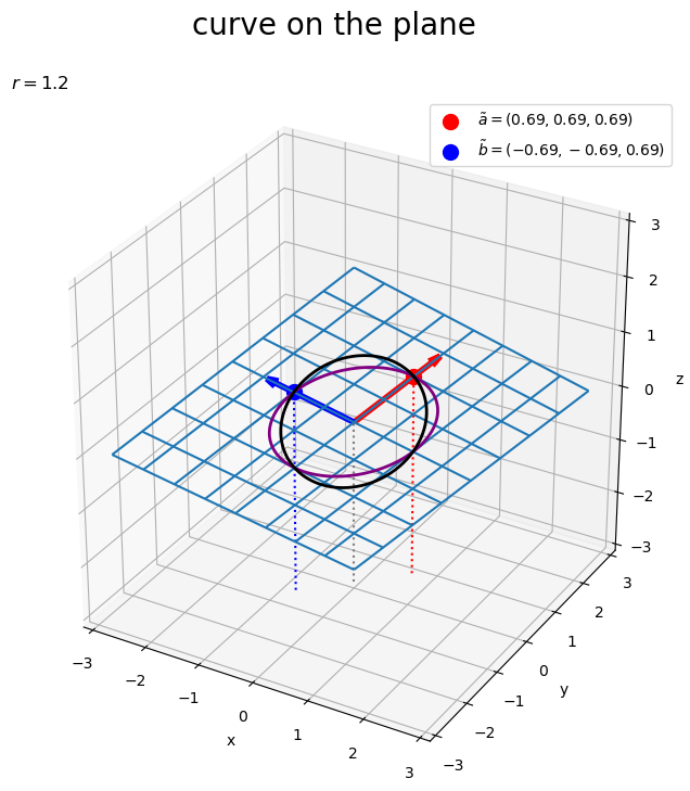
# グラフサイズ用の値を設定
x_min = np.floor(X.min())
x_max = np.ceil(X.max())
y_min = np.floor(Y.min())
y_max = np.ceil(Y.max())
z_min = np.floor(Z.min())
z_max = np.ceil(Z.max())

# 矢のサイズを指定
l = 0.2

# 平面上の2点を結ぶ曲線を作図
fig, ax = plt.subplots(figsize=(8, 8), facecolor='white',
                       subplot_kw={'projection': '3d'})
ax.plot_wireframe(X, Y, Z, zorder=-100) # 平面
ax.quiver(0, 0, 0, *a,
          color='red', linewidth=4, arrow_length_ratio=l/np.linalg.norm(a)) # ベクトルa
ax.quiver(0, 0, 0, *b,
          color='blue', linewidth=4, arrow_length_ratio=l/np.linalg.norm(b)) # ベクトルb
ax.scatter(*tilde_a,
           color='red', s=100,
           label='$\\tilde{a}=('+', '.join(map(str, tilde_a.round(2)))+')$', zorder=100) # ノルムを調整したベクトルaの点
ax.scatter(*tilde_b,
           color='blue', s=100,
           label='$\\tilde{b}=('+', '.join(map(str, tilde_b.round(2)))+')$') # ノルムを調整したベクトルbの点
ax.plot(x, y, z,
        color='purple', linewidth=2, zorder=100) # 2点間の曲線
ax.plot(tilde_x, tilde_y, tilde_z,
        color='black', linewidth=2, zorder=100) # ノルムを調整した2点間の曲線
ax.quiver([0, tilde_a[0], tilde_b[0]],
          [0, tilde_a[1], tilde_b[1]],
          [0, tilde_a[2], tilde_b[2]],
          [0, 0, 0],
          [0, 0, 0],
          [z_min, z_min-tilde_a[2], z_min-tilde_b[2]],
          color=['gray', 'red', 'blue'],
          arrow_length_ratio=0, linestyle=':') # 座標用の補助線
ax.set_xticks(ticks=np.arange(x_min, x_max+0.1))
ax.set_yticks(ticks=np.arange(y_min, y_max+0.1))
ax.set_zticks(ticks=np.arange(z_min, z_max+0.1))
ax.set_zlim(bottom=z_min, top=z_max)
ax.set_xlabel('x')
ax.set_ylabel('y')
ax.set_zlabel('z')
ax.set_title('$r=' + str(r) + '$', loc='left')
fig.suptitle('curve on the plane', fontsize=20)
ax.legend()
ax.set_aspect('equal')
#ax.view_init(elev=90, azim=270) # xy面
#ax.view_init(elev=0, azim=270) # xz面
#ax.view_init(elev=0, azim=0) # yz面
plt.show()
グラフを回転させて確認する。
・作図コード(クリックで展開)
# フレーム数を指定
frame_num = 60

# 水平方向の角度として利用する値を作成
h_n = np.linspace(start=0.0, stop=360.0, num=frame_num+1)[:frame_num]

# グラフオブジェクトを初期化
fig, ax = plt.subplots(figsize=(8, 8), facecolor='white',
                       subplot_kw={'projection': '3d'})
fig.suptitle('curve on the plane', fontsize=20)

# 作図処理を関数として定義
def update(i):

    # 前フレームのグラフを初期化
    plt.cla()

    # i番目の角度を取得
    h = h_n[i]

    # 平面上の2点を結ぶ曲線を作図
    ax.plot_wireframe(X, Y, Z, zorder=-100) # 平面
    ax.quiver(0, 0, 0, *a,
              color='red', linewidth=4, arrow_length_ratio=l/np.linalg.norm(a)) # ベクトルa
    ax.quiver(0, 0, 0, *b,
              color='blue', linewidth=4, arrow_length_ratio=l/np.linalg.norm(b)) # ベクトルb
    ax.scatter(*tilde_a,
               color='red', s=100,
               label='$\\tilde{a}=('+', '.join(map(str, tilde_a.round(2)))+')$', zorder=100) # ノルムを調整したベクトルaの点
    ax.scatter(*tilde_b,
               color='blue', s=100,
               label='$\\tilde{b}=('+', '.join(map(str, tilde_b.round(2)))+')$') # ノルムを調整したベクトルbの点
    ax.plot(x, y, z,
            color='purple', linewidth=2, zorder=100) # 2点間の曲線
    ax.plot(tilde_x, tilde_y, tilde_z,
            color='black', linewidth=2, zorder=100) # ノルムを調整した2点間の曲線
    ax.quiver([0, tilde_a[0], tilde_b[0]],
              [0, tilde_a[1], tilde_b[1]],
              [0, tilde_a[2], tilde_b[2]],
              [0, 0, 0],
              [0, 0, 0],
              [z_min, z_min-tilde_a[2], z_min-tilde_b[2]],
              color=['gray', 'red', 'blue'],
              arrow_length_ratio=0, linestyle=':') # 座標用の補助線
    ax.set_xticks(ticks=np.arange(x_min, x_max+0.1))
    ax.set_yticks(ticks=np.arange(y_min, y_max+0.1))
    ax.set_zticks(ticks=np.arange(z_min, z_max+0.1))
    ax.set_zlim(bottom=z_min, top=z_max)
    ax.set_xlabel('x')
    ax.set_ylabel('y')
    ax.set_zlabel('z')
    ax.set_title('$r=' + str(r) + '$', loc='left')
    ax.legend()
    ax.set_aspect('equal')
    ax.view_init(elev=30, azim=h) # 表示角度

# gif画像を作成
ani = FuncAnimation(fig=fig, func=update, frames=frame_num, interval=100)

# gif画像を保存
ani.save(filename='CurveOnPlane360_3d.gif')
数式からも分かるように、平面も曲線もベクトルを線形結合したものなので、どちらも平行になっているのを確認できる。
ベクトルの値を変化させたアニメーションを作成する。
・作図コード(クリックで展開)
# フレーム数を指定
frame_num = 60

# ノルム(サイズ)を指定
r = 1.2

# 固定するベクトルを指定
a = np.array([1.0, 1.0, 1.0])
tilde_a = r * a / np.linalg.norm(a) # ノルムを調整

# 変化するベクトル用のラジアンを作成
t_n = np.linspace(start=-1.0*np.pi, stop=1.0*np.pi, num=frame_num+1)[:frame_num]
u_n = np.linspace(start=2.0/3.0*np.pi, stop=5.0/3.0*np.pi, num=frame_num+1)[:frame_num]

# 変化するベクトルのサイズを指定
d = 2.0

# 変化するベクトルを作成
b_n = np.array(
    [d * np.sin(t_n) * np.cos(u_n), d * np.sin(t_n) * np.sin(u_n), d * np.cos(t_n)]
).T

# 矢のサイズを指定
l = 0.2

# グラフサイズ用の値を設定
x_min = np.floor(np.min([np.min(Alpha1*tilde_a[0] + Alpha2*b[0]/d) for b in b_n]))
x_max =  np.ceil(np.max([np.max(Alpha1*tilde_a[0] + Alpha2*b[0]/d) for b in b_n]))
y_min = np.floor(np.min([np.min(Alpha1*tilde_a[1] + Alpha2*b[1]/d) for b in b_n]))
y_max =  np.ceil(np.max([np.max(Alpha1*tilde_a[1] + Alpha2*b[1]/d) for b in b_n]))
z_min = np.floor(np.min([np.min(Alpha1*tilde_a[2] + Alpha2*b[2]/d) for b in b_n]))
z_max =  np.ceil(np.max([np.max(Alpha1*tilde_a[2] + Alpha2*b[2]/d) for b in b_n]))

# グラフオブジェクトを初期化
fig, ax = plt.subplots(figsize=(9, 9), facecolor='white',
                       subplot_kw={'projection': '3d'})
fig.suptitle('curve on the plane', fontsize=20)

# 作図処理を関数として定義
def update(i):

    # 前フレームのグラフを初期化
    plt.cla()

    # i番目のベクトルを取得
    b = b_n[i]
    tilde_b = r * b / np.linalg.norm(b) # ノルムを調整

    # ベクトルa,bのなす角を計算
    theta = np.arccos(np.dot(a, b) / np.linalg.norm(a) / np.linalg.norm(b))

    # 2点間の曲線の座標を計算
    x = beta1 * tilde_a[0] + beta2 * tilde_b[0]
    y = beta1 * tilde_a[1] + beta2 * tilde_b[1]
    z = beta1 * tilde_a[2] + beta2 * tilde_b[2]

    # 点ごとにノルムを計算
    norm_xyz = np.linalg.norm(np.stack([x, y, z], axis=1), axis=1)

    # ノルムを一定に調整
    tilde_x = r * x / norm_xyz
    tilde_y = r * y / norm_xyz
    tilde_z = r * z / norm_xyz

    # 平面の座標を計算
    X = Alpha1 * tilde_a[0] + Alpha2 * tilde_b[0]
    Y = Alpha1 * tilde_a[1] + Alpha2 * tilde_b[1]
    Z = Alpha1 * tilde_a[2] + Alpha2 * tilde_b[2]

    # 平面上の2点を結ぶ曲線を作図
    ax.plot_wireframe(X, Y, Z, zorder=-100) # 平面
    ax.quiver(0, 0, 0, *a,
              color='red', linewidth=4, arrow_length_ratio=l/np.linalg.norm(a)) # ベクトルa
    ax.quiver(0, 0, 0, *b,
              color='blue', linewidth=4, arrow_length_ratio=l/np.linalg.norm(b)) # ベクトルb
    ax.scatter(*tilde_a,
               color='red', s=100,
               label='$\\tilde{a}=('+', '.join(map(str, tilde_a.round(2)))+')$', zorder=100) # ノルムを調整したベクトルaの点
    ax.scatter(*tilde_b,
               color='blue', s=100,
               label='$\\tilde{b}=('+', '.join(map(str, tilde_b.round(2)))+')$') # ノルムを調整したベクトルbの点
    ax.plot(x, y, z,
            color='purple', linewidth=2, zorder=100) # 2点間の曲線
    ax.plot(tilde_x, tilde_y, tilde_z,
            color='black', linewidth=2, zorder=100) # ノルムを調整した2点間の曲線
    ax.quiver([0, tilde_a[0], tilde_b[0]],
              [0, tilde_a[1], tilde_b[1]],
              [0, tilde_a[2], tilde_b[2]],
              [0, 0, 0],
              [0, 0, 0],
              [z_min, z_min-tilde_a[2], z_min-tilde_b[2]],
              color=['gray', 'red', 'blue'],
              arrow_length_ratio=0, linestyle=':') # 座標用の補助線
    ax.set_xticks(ticks=np.arange(x_min, x_max+0.1))
    ax.set_yticks(ticks=np.arange(y_min, y_max+0.1))
    ax.set_zticks(ticks=np.arange(z_min, z_max+0.1))
    ax.set_xlim(left=x_min, right=x_max)
    ax.set_ylim(bottom=y_min, top=y_max)
    ax.set_zlim(bottom=z_min, top=z_max)
    ax.set_xlabel('x')
    ax.set_ylabel('y')
    ax.set_zlabel('z')
    ax.set_title('$r=' + str(r) + ', ' +
                 '\\theta=' + str((theta/np.pi).round(2)) + '\pi$', loc='left')
    ax.legend(loc='upper left')
    ax.set_aspect('equal')

# gif画像を作成
ani = FuncAnimation(fig=fig, func=update, frames=frame_num, interval=100)

# gif画像を保存
ani.save(filename='CurveOnPlane_3d.gif')
この平面は、「球面上で可視化」における球の断面を拡張した平面である。
この記事では、3次元空間において良い感じの曲線を引けた。
おわりに
一度諦めたことができるようになりました。その嬉しさをなんとか伝えたい思いで(?)、4節も使って(ほぼ同じ内容を)解説しています。
この記事の投稿日に公開された歌唱動画を聴きましょう。
まーちゃんの供給が盛りだくさんで浮かれ気分な今日この頃です。