はじめに
『スタンフォード ベクトル・行列からはじめる最適化数学』の学習ノートです。
「数式の行間埋め」や「Pythonを使っての再現」によって理解を目指します。本と一緒に読んでください。
この記事は3.2節「距離」の内容です。
ベクトルのユークリッド距離を可視化します。
【前の内容】
【他の内容】
【今回の内容】
距離の可視化
ユークリッド距離(euclidean distance)をグラフで確認します。
利用するライブラリ読み込みます。
# 利用ライブラリ
import numpy as np
import matplotlib.pyplot as plt
from matplotlib.animation import FuncAnimation
2次元の場合
まずは、2次元空間(平面)上でベクトルの長さ(2点の距離)を可視化します。
2つの2次元ベクトルを指定します。
# 2点の座標(ベクトル)を指定
a = np.array([1.0, 2.0])
b = np.array([3.0, 3.0])
を
a、を
bとして値を指定します。ただし、Pythonでは0からインデックスが割り当てられるので、の値は
a[0]に対応します。
2次元空間上のベクトルと座標の関係を確認します。
# 作図用の値を設定
x_min = np.floor(np.min([0.0, a[0], b[0]])) - 1
x_max = np.ceil(np.max([0.0, a[0], b[0]])) + 1
y_min = np.floor(np.min([0.0, a[1], b[1]])) - 1
y_max = np.ceil(np.max([0.0, a[1], b[1]])) + 1

# 2Dベクトル差を作図
fig, ax = plt.subplots(figsize=(6, 6), facecolor='white')
ax.scatter(0, 0, c='orange', s=100) # 原点
ax.scatter(*a, c='red', s=100) # 点a
ax.scatter(*b, c='blue', s=100) # 点b
ax.quiver(*a, *-a, color='red', label='-a',
          angles='xy', scale_units='xy', scale=1) # ベクトル-a
ax.quiver(0, 0, *b, color='blue', label='b',
          angles='xy', scale_units='xy', scale=1) # ベクトルb
ax.quiver(*a, *b-a, color='purple', label='b-a',
          angles='xy', scale_units='xy', scale=1) # ベクトルb-a
ax.annotate(xy=[0, 0], text='O', size=15, ha='right', va='top') # 原点ラベル
ax.annotate(xy=a, text='a', size=15, ha='right', va='bottom') # 点aラベル
ax.annotate(xy=b, text='b', size=15, ha='right', va='bottom') # 点bラベル
ax.set_xticks(ticks=np.arange(x_min, x_max+1))
ax.set_yticks(ticks=np.arange(y_min, y_max+1))
ax.grid()
ax.set_xlabel('x')
ax.set_ylabel('y')
ax.set_title('a=('+', '.join(map(str, a))+'), ' +
             'b=('+', '.join(map(str, b))+')', loc='left')
fig.suptitle('vector b-a', fontsize=20)
ax.legend()
ax.set_aspect('equal')
plt.show()

ベクトルのグラフを
axes.quiver()で描画します。第1・2引数に始点の座標、第3・4引数にベクトルのサイズ(変化量)を指定します。この例では、原点を始点とします。
配列a, bの前に*を付けてアンパック(展開)して指定しています。
点から点
への移動は、ベクトル
で表わせるのでした(1.2節)。
のノルムを計算して、ベクトルを描画します。
# 作図用の値を設定
x_min = np.floor(np.min([a[0], b[0]])) - 1
x_max = np.ceil(np.max([a[0], b[0]])) + 1
y_min = np.floor(np.min([a[1], b[1]])) - 1
y_max = np.ceil(np.max([a[1], b[1]])) + 1

# 距離を計算
dist_ab = np.sqrt(np.sum((b - a)**2))
print(dist_ab)
dist_ab = np.sqrt(np.dot(b-a, b-a))
print(dist_ab)
dist_ab = (np.linalg.norm(b - a))
print(dist_ab)

# 2Dベクトルを作図
fig, ax = plt.subplots(figsize=(6, 5), facecolor='white')
ax.scatter(*a, c='red', s=100, label='a') # 始点
ax.scatter(*b, c='blue', s=100, label='b') # 終点
ax.quiver(*a, *(b-a), angles='xy', scale_units='xy', scale=1) # ベクトルb-a
ax.annotate(xy=0.5*(a+b), text='b - a', size=15, ha='right', va='bottom') # ベクトルb-aラベル
ax.set_xticks(ticks=np.arange(x_min, x_max+1))
ax.set_yticks(ticks=np.arange(y_min, y_max+1))
ax.grid()
ax.set_xlabel('x')
ax.set_ylabel('y')
ax.set_title('$a=('+', '.join(map(str, a))+'), ' +
             'b=('+', '.join(map(str, b))+'), ' +
             '\\|b-a\\| = '+str(dist_ab.round(2))+'$', loc='left')
fig.suptitle('dist a, b', fontsize=20)
ax.legend()
ax.set_aspect('equal')
plt.show()
2.23606797749979
2.23606797749979
2.23606797749979

ユークリッド距離(差のユークリッドノルム)を計算して、タイトルに表示します。
平方根はnp.sqrt()、内積はnp.dot()で計算できます。また、ノルムはnp.linalg.norm()でも計算できます。
同様に、のノルムを計算して、作図します。
# 距離を計算
dist_ba = np.sqrt(np.sum((a - b)**2))
print(dist_ba)
dist_ba = np.sqrt(np.dot(a-b, a-b))
print(dist_ba)
dist_ba = (np.linalg.norm(a - b))
print(dist_ba)

# 2Dベクトルを作図
fig, ax = plt.subplots(figsize=(6, 5), facecolor='white')
ax.scatter(*a, c='red', s=100, label='a') # 始点
ax.scatter(*b, c='blue', s=100, label='b') # 終点
ax.quiver(*b, *(a-b), angles='xy', scale_units='xy', scale=1) # ベクトルa-b
ax.annotate(xy=0.5*(a+b), text='a - b', size=15, ha='right', va='bottom') # ベクトルa-bラベル
ax.set_xticks(ticks=np.arange(x_min, x_max+1))
ax.set_yticks(ticks=np.arange(y_min, y_max+1))
ax.grid()
ax.set_xlabel('x')
ax.set_ylabel('y')
ax.set_title('$a=('+', '.join(map(str, a))+'), ' +
             'b=('+', '.join(map(str, b))+'), ' +
             '\\|b-a\\| = '+str(dist_ba.round(2))+'$', loc='left')
fig.suptitle('dist b, a', fontsize=20)
ax.legend()
ax.set_aspect('equal')
plt.show()
2.23606797749979
2.23606797749979
2.23606797749979
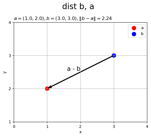
符号を反転(ベクトルの向きを反対)しても距離(ノルム)が変わらないのが分かります。
ベクトルを直角三角形の斜辺としたときの、3辺の関係を確認します。
作図コード(クリックで展開)
# 2Dベクトルを作図
fig, ax = plt.subplots(figsize=(6, 6), facecolor='white')
ax.scatter(*a, c='red', s=100, label='a') # 点a
ax.scatter(*b, c='blue', s=100, label='b') # 点b
ax.quiver(*a, *(b-a), angles='xy', scale_units='xy', scale=1) # ベクトルb-a
ax.plot([a[0], b[0], b[0]], [a[1], a[1], b[1]],
        color='black', linewidth=1.5) # 底辺と高さ
ax.plot([[0, a[0]], [a[0], a[0]]], [[a[1], 0], [a[1], a[1]]],
       color='red', linewidth=1.5, linestyle=':') # aに関する長さ
ax.plot([[0, b[0]], [b[0], b[0]]], [[b[1], 0], [b[1], b[1]]],
       color='blue', linewidth=1.5, linestyle=':') # bに関する長さ
ax.annotate(xy=0.5*(a+b), text='$\sqrt{(b_1-a_1)^2+(b_2-a_2)^2}$', size=10, ha='right', va='bottom') # ベクトルb-aラベル
ax.annotate(xy=[0.5*(a[0]+b[0]), a[1]], text='$b_1-a_1$', size=15, ha='center', va='top') # 底辺ラベル
ax.annotate(xy=[b[0], 0.5*(a[1]+b[1])], text='$b_2-a_2$', size=15, ha='left', va='center') # 高さラベル
ax.annotate(xy=[0.5*a[0], a[1]], text='$a_1$', color='red', size=15, ha='center', va='top') # a1ラベル
ax.annotate(xy=[a[0], 0.5*a[1]], text='$a_2$', color='red', size=15, ha='left', va='center') # a2ラベル
ax.annotate(xy=[0.5*b[0], b[1]], text='$b_1$', color='blue', size=15, ha='center', va='bottom') # b1ラベル
ax.annotate(xy=[b[0], 0.5*b[1]], text='$b_2$', color='blue', size=15, ha='left', va='center') # b2ラベル
ax.set_xticks(ticks=np.arange(np.min([0.0, x_min]), x_max+1))
ax.set_yticks(ticks=np.arange(np.min([0.0, y_min]), y_max+1))
ax.set_xlim(left=np.min([0.0, x_min]), right=x_max)
ax.set_ylim(bottom=np.min([0.0, y_min]), top=y_max)
ax.grid()
ax.set_xlabel('x')
ax.set_ylabel('y')
ax.set_title('$a=('+', '.join(map(str, a))+'), ' +
             'b=('+', '.join(map(str, b))+'), ' +
             '\\|b-a\\| = '+str(dist_ab.round(2))+'$', loc='left')
fig.suptitle('dist a, b', fontsize=20)
ax.legend()
ax.set_aspect('equal')
plt.show()

y軸(の垂直線)と点
との距離は
で、点
との距離は
です。よって、底辺(黒色の実線)は、水平方向の青色の点線から赤色の点線を引いた線分なので、
です。
同様に、x軸(の水平線)と点
との距離は
、点
との距離は
なので、高さ(黒色の実線)は、
です。
底辺が、高さが
なので、三平方の定理より斜辺が
になるのが分かります。
ベクトルの値を変化させたアニメーションを作成します。
・作図コード(クリックで展開)
# フレーム数を設定
frame_num = 51

# ベクトルとして利用する値を指定
a_vals = np.array(
    [np.linspace(start=-6.0, stop=6.0, num=frame_num),
     np.linspace(start=0.0, stop=10.0, num=frame_num)]
).T
b_vals = np.array(
    [np.linspace(start=3.0, stop=3.0, num=frame_num),
     np.linspace(start=3.0, stop=3.0, num=frame_num)]
).T

# 作図用の値を設定
x_min = np.floor(np.min([*a_vals[:, 0], *b_vals[:, 0]])) - 1
x_max = np.ceil(np.max([*a_vals[:, 0], *b_vals[:, 0]])) + 1
y_min = np.floor(np.min([*a_vals[:, 1], *b_vals[:, 1]])) - 1
y_max = np.ceil(np.max([*a_vals[:, 1], *b_vals[:, 1]])) + 1

# 作図用のオブジェクトを初期化
fig, ax = plt.subplots(figsize=(6, 5), facecolor='white')
fig.suptitle('dist a, b', fontsize=20)

# 作図処理を関数として定義
def update(i):

    # 前フレームのグラフを初期化
    plt.cla()

    # i番目のベクトルを作成
    a = a_vals[i]
    b = b_vals[i]

    # 距離を計算
    dist_ab = (np.linalg.norm(b - a))

    # 2Dベクトルを作図
    ax.scatter(*a, c='red', s=100, label='a') # 始点
    ax.scatter(*b, c='blue', s=100, label='b') # 終点
    ax.quiver(*a, *(b-a), angles='xy', scale_units='xy', scale=1) # ベクトルb-a
    ax.annotate(xy=0.5*(a+b), text='b - a', size=15, ha='right', va='bottom') # ベクトルb-aラベル
    ax.set_xticks(ticks=np.arange(x_min, x_max+1))
    ax.set_yticks(ticks=np.arange(y_min, y_max+1))
    ax.grid()
    ax.set_xlabel('x')
    ax.set_ylabel('y')
    ax.set_title('$a=('+', '.join(map(str, a.round(2)))+'), ' +
                 'b=('+', '.join(map(str, b.round(2)))+'), ' +
                 '\\|b-a\\| = '+str(dist_ab.round(2))+'$', loc='left')
    fig.suptitle('dist a, b', fontsize=20)
    ax.legend()
    ax.set_aspect('equal')

# gif画像を作成
ani = FuncAnimation(fig=fig, func=update, frames=frame_num, interval=100)

# gif画像を保存
ani.save('dist_2d.gif')
作図処理をupdate()として定義して、FuncAnimation()でgif画像を作成します。

3次元の場合
続いて、3次元空間上でベクトルの差を可視化します。
3次元ベクトルを指定します。
# 2点の座標(ベクトル)を指定
a = np.array([1.0, 2.0, 3.0])
b = np.array([4.0, 4.0, 4.0])
を
a、を
bとして値を指定します。
3次元空間上のベクトルと座標の関係を確認します。
# 作図用の値を設定
x_min = np.floor(np.min([0.0, a[0], b[0]])) - 1
x_max = np.ceil(np.max([0.0, a[0], b[0]])) + 1
y_min = np.floor(np.min([0.0, a[1], b[1]])) - 1
y_max = np.ceil(np.max([0.0, a[1], b[1]])) + 1
z_min = np.floor(np.min([0.0, a[2], b[2]])) - 1
z_max = np.ceil(np.max([0.0, a[2], b[2]])) + 1

# 3Dベクトル差を作図
fig, ax = plt.subplots(figsize=(7, 7), facecolor='white',
                       subplot_kw={'projection': '3d'})
ax.quiver(*a, *-a, color='red', label='-a', arrow_length_ratio=0.1) # ベクトル-a
ax.quiver(0, 0, 0, *b, color='blue', label='b', arrow_length_ratio=0.1) # ベクトルb
ax.quiver(*a, *b-a, color='purple', label='b-a', arrow_length_ratio=0.1) # ベクトルb-a
ax.scatter(0, 0, 0, c='orange', s=100) # 原点
ax.scatter(*a, c='red', s=100) # 点a
ax.scatter(*b, c='blue', s=100) # 点b
ax.text(0, 0, 0, s='O', size=15, ha='right', va='top', zorder=20) # 原点ラベル
ax.text(*a, s='a', size=15, ha='right', va='bottom', zorder=20) # 点aラベル
ax.text(*b, s='b', size=15, ha='left', va='top', zorder=20) # 点bラベル
ax.quiver([0, a[0], b[0]], [0, a[1], b[1]], [z_min, z_min, z_min],
          [0, 0, 0], [0, 0, 0], [-z_min, a[2]-z_min, b[2]-z_min],
          color='gray', arrow_length_ratio=0, linestyle=':') # 補助線
ax.set_xticks(ticks=np.arange(x_min, x_max+1))
ax.set_yticks(ticks=np.arange(y_min, y_max+1))
ax.set_zticks(ticks=np.arange(z_min, z_max+1))
ax.set_zlim(z_min, z_max)
ax.set_xlabel('x')
ax.set_ylabel('y')
ax.set_zlabel('z')
ax.set_title('a=('+', '.join(map(str, a))+'), ' +
             'b=('+', '.join(map(str, b))+')', loc='left')
fig.suptitle('point a, b', fontsize=20)
ax.legend()
ax.set_aspect('equal')
plt.show()

axes.quiver()の第1・2・3引数に始点の座標、第4・5・6引数にベクトルのサイズを指定します。この例では、原点を始点とします。
のノルムを計算して、ベクトルを描画します。
# 作図用の値を設定
x_min = np.floor(np.min([a[0], b[0]])) - 1
x_max = np.ceil(np.max([a[0], b[0]])) + 1
y_min = np.floor(np.min([a[1], b[1]])) - 1
y_max = np.ceil(np.max([a[1], b[1]])) + 1
z_min = np.floor(np.min([a[2], b[2]])) - 1
z_max = np.ceil(np.max([a[2], b[2]])) + 1

# 距離を計算
dist_ab = np.sqrt(np.sum((b - a)**2))
print(dist_ab)
dist_ab = np.sqrt(np.dot(b-a, b-a))
print(dist_ab)
dist_ab = (np.linalg.norm(b - a))
print(dist_ab)

# 3Dベクトル差を作図
fig, ax = plt.subplots(figsize=(7, 7), facecolor='white',
                       subplot_kw={'projection': '3d'})
ax.quiver(*a, *b-a, color='black', arrow_length_ratio=0.1) # ベクトルb-a
ax.scatter(*a, c='red', s=100, label='a') # 点a
ax.scatter(*b, c='blue', s=100, label='b') # 点b
ax.text(*0.5*(a+b), s='b - a', size=15, ha='right', va='bottom', zorder=20) # ベクトルb-aラベル
ax.quiver([a[0], b[0]], [a[1], b[1]], [z_min, z_min],
          [0, 0], [0, 0], [a[2]-z_min, b[2]-z_min],
          color='gray', arrow_length_ratio=0, linestyle=':') # 補助線
ax.set_xticks(ticks=np.arange(x_min, x_max+1))
ax.set_yticks(ticks=np.arange(y_min, y_max+1))
ax.set_zticks(ticks=np.arange(z_min, z_max+1))
ax.set_zlim(z_min, z_max)
ax.set_xlabel('x')
ax.set_ylabel('y')
ax.set_zlabel('z')
ax.set_title('$a=('+', '.join(map(str, a))+'), ' +
             'b=('+', '.join(map(str, b))+'), ' +
             '\\|b-a\\| = '+str(dist_ab.round(2))+'$', loc='left')
fig.suptitle('dist a, b', fontsize=20)
ax.legend()
ax.set_aspect('equal')
plt.show()
3.7416573867739413
3.7416573867739413
3.7416573867739413

「2次元の場合」と同じコードでノルムを計算できます。
同様に、のノルムを計算して、作図します。
# 距離を計算
dist_ba = np.sqrt(np.sum((a - b)**2))
print(dist_ba)
dist_ba = np.sqrt(np.dot(a-b, a-b))
print(dist_ba)
dist_ba = (np.linalg.norm(a - b))
print(dist_ba)

# 3Dベクトル差を作図
fig, ax = plt.subplots(figsize=(7, 7), facecolor='white',
                       subplot_kw={'projection': '3d'})
ax.quiver(*b, *a-b, color='black', arrow_length_ratio=0.1) # ベクトルb-a
ax.scatter(*a, c='red', s=100, label='a') # 点a
ax.scatter(*b, c='blue', s=100, label='b') # 点b
ax.text(*0.5*(a+b), s='a - b', size=15, ha='right', va='bottom', zorder=20) # ベクトルb-aラベル
ax.quiver([a[0], b[0]], [a[1], b[1]], [z_min, z_min],
          [0, 0], [0, 0], [a[2]-z_min, b[2]-z_min],
          color='gray', arrow_length_ratio=0, linestyle=':') # 補助線
ax.set_xticks(ticks=np.arange(x_min, x_max+1))
ax.set_yticks(ticks=np.arange(y_min, y_max+1))
ax.set_zticks(ticks=np.arange(z_min, z_max+1))
ax.set_zlim(z_min, z_max)
ax.set_xlabel('x')
ax.set_ylabel('y')
ax.set_zlabel('z')
ax.set_title('$a=('+', '.join(map(str, a))+'), ' +
             'b=('+', '.join(map(str, b))+'), ' +
             '\\|a-b\\| = '+str(dist_ba.round(2))+'$', loc='left')
fig.suptitle('dist b, a', fontsize=20)
ax.legend()
ax.set_aspect('equal')
plt.show()
3.7416573867739413
3.7416573867739413
3.7416573867739413

2点間の距離は変わりません。
ベクトルを直角三角形の斜辺としたときの、3辺の関係を確認します。
作図コード(クリックで展開)
# 3Dベクトル差を作図
fig, ax = plt.subplots(figsize=(7, 7), facecolor='white',
                       subplot_kw={'projection': '3d'})
ax.scatter(*a, c='red', s=100, label='a') # 点a
ax.scatter(*b, c='blue', s=100, label='b') # 点b
ax.quiver(*a, *b-a, color='black', arrow_length_ratio=0.1) # ベクトルb-a
ax.quiver(*a, b[0]-a[0], b[1]-a[1], 0, color='black', arrow_length_ratio=0.00) # 底辺の斜辺
ax.quiver([a[0], a[0], a[0], a[0]], [a[1], b[1], a[1], b[1]], [a[2], a[2], b[2], b[2]],
          [b[0]-a[0], b[0]-a[0], b[0]-a[0], b[0]-a[0]], [0, 0, 0, 0], [0, 0, 0, 0],
          color='gray', arrow_length_ratio=0.0) # 横幅
ax.quiver([a[0], b[0], a[0], b[0]], [a[1], a[1], a[1], a[1]], [a[2], a[2], b[2], b[2]],
          [0, 0, 0, 0], [b[1]-a[1], b[1]-a[1], b[1]-a[1], b[1]-a[1]], [0, 0, 0, 0],
          color='gray', arrow_length_ratio=0.0) # 奥行き
ax.quiver([a[0], b[0], a[0], b[0]], [a[1], a[1], b[1], b[1]], [a[2], a[2], a[2], a[2]],
          [0, 0, 0, 0], [0, 0, 0, 0], [b[2]-a[2], b[2]-a[2], b[2]-a[2], b[2]-a[2]],
          color='gray', arrow_length_ratio=0.0) # 高さ
ax.quiver([a[0], a[0], a[0]], [a[1], a[1], a[1]], [a[2], a[2], a[2]],
          [-a[0], 0, 0], [0, -a[1], 0], [0, 0, -a[2]],
          color='red', arrow_length_ratio=0, linestyle=':') # aに関する長さ
ax.quiver([b[0], b[0], b[0]], [b[1], b[1], b[1]], [b[2], b[2], b[2]],
          [-b[0], 0, 0], [0, -b[1], 0], [0, 0, -b[2]],
          color='blue', arrow_length_ratio=0, linestyle=':') # bに関する長さ
ax.text(*0.5*(a+b), s='$\sqrt{(b_1-a_1)^2 + (b_2-a_2)^2 + (b_3-a_3)^2}$',
        size=7, ha='center', va='bottom', zorder=20) # 斜辺ラベル
ax.text(0.5*(a[0]+b[0]), 0.5*(a[1]+b[1]), a[2], s='$\sqrt{(b_1-a_1)^2 + (b_2-a_2)^2}$',
        size=7, ha='center', va='top', zorder=20) # 底辺の斜辺ラベル
ax.text(0.5*(a[0]+b[0]), a[1], a[2], s='$b_1-a_1$', size=10, ha='center', va='top') # 横幅ラベル
ax.text(b[0], 0.5*(a[1]+b[1]), a[2], s='$b_2-a_2$', size=10, ha='center', va='center') # 奥行きラベル
ax.text(b[0], b[1], 0.5*(a[2]+b[2]), s='$b_3-a_3$', size=10, ha='left', va='center') # 高さラベル
ax.text(0.5*a[0], a[1], a[2], s='$a_1$', color='red', size=10, ha='center', va='bottom') # a1ラベル
ax.text(a[0], 0.5*a[1], a[2], s='$a_2$', color='red', size=10, ha='left', va='center') # a2ラベル
ax.text(a[0], a[1], 0.5*a[2], s='$a_3$', color='red', size=10, ha='left', va='center') # a3ラベル
ax.text(0.5*b[0], b[1], b[2], s='$b_1$', color='blue', size=10, ha='center', va='bottom') # b1ラベル
ax.text(b[0], 0.5*b[1], b[2], s='$b_2$', color='blue', size=10, ha='right', va='bottom') # b2ラベル
ax.text(b[0], b[1], 0.5*b[2], s='$b_3$', color='blue', size=10, ha='left', va='center') # b3ラベル
ax.set_xticks(ticks=np.arange(np.min([0.0, x_min]), x_max+1))
ax.set_yticks(ticks=np.arange(np.min([0.0, y_min]), y_max+1))
ax.set_zticks(ticks=np.arange(np.min([0.0, z_min]), z_max+1))
ax.set_xlabel('x')
ax.set_ylabel('y')
ax.set_zlabel('z')
ax.set_title('$a=('+', '.join(map(str, a))+'), ' +
             'b=('+', '.join(map(str, b))+'), ' +
             '\\|b-a\\| = '+str(dist_ab.round(2))+'$', loc='left')
fig.suptitle('dist a, b', fontsize=20)
ax.legend()
ax.set_aspect('equal')
plt.show()

「2次元の場合」と同様に、横幅・奥行き・高さは、青色の点線と赤色の点線
の差
です。
三平方の定理より、横幅がで奥行きが
なので底辺上の斜辺が
であり、また高さが
なので直方体の対角線が
になるのが分かります。
ベクトルの値を変化させたアニメーションを作成します。
・作図コード(クリックで展開)
# フレーム数を設定
frame_num = 51

# ベクトルとして利用する値を指定
a_vals = np.array(
    [np.linspace(start=-6.0, stop=6.0, num=frame_num),
     np.linspace(start=0.0, stop=10.0, num=frame_num),
     np.linspace(start=-2.0, stop=3.0, num=frame_num)]
).T
b_vals = np.array(
    [np.linspace(start=3.0, stop=3.0, num=frame_num),
     np.linspace(start=3.0, stop=3.0, num=frame_num),
     np.linspace(start=3.0, stop=3.0, num=frame_num)]
).T

# 作図用の値を設定
x_min = np.floor(np.min([*a_vals[:, 0], *b_vals[:, 0]])) - 1
x_max = np.ceil(np.max([*a_vals[:, 0], *b_vals[:, 0]])) + 1
y_min = np.floor(np.min([*a_vals[:, 1], *b_vals[:, 1]])) - 1
y_max = np.ceil(np.max([*a_vals[:, 1], *b_vals[:, 1]])) + 1
z_min = np.floor(np.min([*a_vals[:, 2], *b_vals[:, 2]])) - 1
z_max = np.ceil(np.max([*a_vals[:, 2], *b_vals[:, 2]])) + 1

# 作図用のオブジェクトを初期化
fig, ax = plt.subplots(figsize=(8, 8), facecolor='white',
                       subplot_kw={'projection': '3d'})
fig.suptitle('dist a, b', fontsize=20)

# 作図処理を関数として定義
def update(i):

    # 前フレームのグラフを初期化
    plt.cla()

    # i番目のベクトルを作成
    a = a_vals[i]
    b = b_vals[i]

    # 距離を計算
    dist_ab = (np.linalg.norm(b - a))

    # 3Dベクトル差を作図
    ax.quiver(*a, *b-a, color='black', arrow_length_ratio=0.1) # ベクトルb-a
    ax.scatter(*a, c='red', s=100, label='a') # 点a
    ax.scatter(*b, c='blue', s=100, label='b') # 点b
    ax.text(*0.5*(a+b), s='b - a', size=15, ha='right', va='bottom', zorder=20) # ベクトルb-aラベル
    ax.quiver([x_min, x_min, a[0], b[0], a[0], b[0]],
              [a[1], b[1], y_max, y_max, a[1], b[1]],
              [a[2], b[2], a[2], b[2], z_min, z_min],
              [a[0]-x_min, b[0]-x_min, 0, 0, 0, 0],
              [0, 0, a[1]-y_max, b[1]-y_max, 0, 0],
              [0, 0, 0, 0, a[2]-z_min, b[2]-z_min],
              color='gray', arrow_length_ratio=0, linestyle=':') # 補助線
    ax.set_xticks(ticks=np.arange(x_min, x_max+1))
    ax.set_yticks(ticks=np.arange(y_min, y_max+1))
    ax.set_zticks(ticks=np.arange(z_min, z_max+1))
    ax.set_xlim(x_min, x_max)
    ax.set_ylim(y_min, y_max)
    ax.set_zlim(z_min, z_max)
    ax.set_xlabel('x')
    ax.set_ylabel('y')
    ax.set_zlabel('z')
    ax.set_title('$a=('+', '.join(map(str, a.round(2)))+'), ' +
                 'b=('+', '.join(map(str, b.round(2)))+'), ' +
                 '\\|b-a\\| = '+str(dist_ab.round(2))+'$', loc='left')
    fig.suptitle('dist a, b', fontsize=20)
    ax.legend()
    ax.set_aspect('equal')

# gif画像を作成
ani = FuncAnimation(fig=fig, func=update, frames=frame_num, interval=100)

# gif画像を保存
ani.save('dist_3d.gif')
この記事では、ユークリッド距離を可視化しました。次の記事では、距離を用いた例を確認します。
参考書籍
- Stephen Boyd・Lieven Vandenberghe(著),玉木 徹(訳)『スタンフォード ベクトル・行列からはじめる最適化数学』講談社サイエンティク,2021年.
おわりに
このシリーズでは1記事に収める内容をいつもより細かくしているのですが、その分記事数が増えて1記事での説明が薄くなっていしまいます。他の記事とセットで読む方が分かりやすかったりするので(例えばノルムと距離とか)、ぜひ別の記事も読んでみてください。
【次の内容】