はじめに
Matplotlibライブラリを利用して、を作成します。
【前の内容】
【目次】
傾いた3次元格子の作図
前回は、Matplotlibライブラリを利用して、3次元空間上に直方体の格子のグラフを作成します。
今回は、3次元空間上に平行六面体の格子のグラフを作成します。前回と「2次元格子の作図【Matplotlib】 - からっぽのしょこ」の記事も参照してください。
利用するライブラリを読み込みます。
# 利用ライブラリ
import numpy as np
import matplotlib.pyplot as plt
from matplotlib.animation import FuncAnimation
3次元格子の描画
3次元の格子(平行六面体の立体)の作図方法を確認します。
x軸・y軸・z軸の値を作成します。(説明に数式を使いますが、特に重要なわけではないので読み飛ばしてください。)
# 点の座標を指定
p = np.array([1.0, 1.0, 1.0])
q = np.array([1.0, -1.0, -1.0])
r = np.array([-1.0, 1.0, -1.0])

# 立体用の係数を指定
a = np.arange(start=0.0, stop=4.1, step=1.0)
b = np.arange(start=0.0, stop=3.1, step=1.0)
c = np.arange(start=0.0, stop=2.1, step=1.0)
print(a)
print(b)
print(c)
print(a.shape)
print(b.shape)
print(c.shape)

# 係数の格子点を作成
A, B, C = np.meshgrid(a, b, c)
print(A.shape)
print(B.shape)

# 立体の座標を計算
X = A * p[0] + B * q[0] + C * r[0]
Y = A * p[1] + B * q[1] + C * r[1]
Z = A * p[2] + B * q[2] + C * r[2]
print(X[0])
print(Y[0])
print(Z[0])
[0. 1. 2. 3. 4.]
[0. 1. 2. 3.]
[0. 1. 2.]
(5,)
(4,)
(3,)
(4, 5, 3)
(4, 5, 3)
[[ 0. -1. -2.]
 [ 1.  0. -1.]
 [ 2.  1.  0.]
 [ 3.  2.  1.]
 [ 4.  3.  2.]]
[[0. 1. 2.]
 [1. 2. 3.]
 [2. 3. 4.]
 [3. 4. 5.]
 [4. 5. 6.]]
[[ 0. -1. -2.]
 [ 1.  0. -1.]
 [ 2.  1.  0.]
 [ 3.  2.  1.]
 [ 4.  3.  2.]]
点・点
・点
の座標(x軸の値
・y軸の値
・z軸の値
)を
p, q, rとして指定します。Pythonのインデックスに合わせて、添字を0から割り当てています。
立体の座標計算に使う係数の値を
a, b, cとして作成して、格子状の点(全ての組み合わせ)をnp.meshgrid()で作成してA, B, Cとします。
平面のx軸の値・y軸の値
・z軸の値
を計算して、
X, Y, Zとします。
X, Y, Zを用いて、散布図を作成してプロット位置を確認します。
# 3D格子点を作図
fig, ax = plt.subplots(figsize=(7, 7), facecolor='white',
                       subplot_kw={'projection': '3d'})
ax.scatter(X, Y, Z) # 格子点
ax.quiver(0, 0, 0, p[0], p[1], p[2],
          color='limegreen', linewidth=4, arrow_length_ratio=0.0) # pに関する直線
ax.quiver(0, 0, 0, q[0], q[1], q[2],
          color='burlywood', linewidth=4, arrow_length_ratio=0.0) # qに関する直線
ax.quiver(0, 0, 0, r[0], r[1], r[2],
          color='aqua', linewidth=4, arrow_length_ratio=0.0) # rに関する直線
ax.scatter(p[0], p[1], p[2],
           color='limegreen', s=100,
           label='p=('+', '.join(map(str, p.round(2)))+')') # 点p
ax.scatter(q[0], q[1], q[2],
           color='burlywood', s=100,
           label='q=('+', '.join(map(str, q.round(2)))+')') # 点q
ax.scatter(r[0], r[1], r[2],
           color='aqua', s=100,
           label='r=('+', '.join(map(str, r.round(2)))+')') # 点r
ax.scatter(0, 0, 0,
           color='orange', s=100, label='O=(0, 0, 0)') # 原点
ax.set_xlabel('x')
ax.set_ylabel('y')
ax.set_zlabel('z')
fig.suptitle('Axes.scatter(X, Y, Z)', fontsize=20)
ax.legend()
ax.set_aspect('equal')
#ax.view_init(elev=90, azim=270) # xy面
#ax.view_init(elev=0, azim=270) # xz面
#ax.view_init(elev=0, azim=0) # yz面
plt.show()
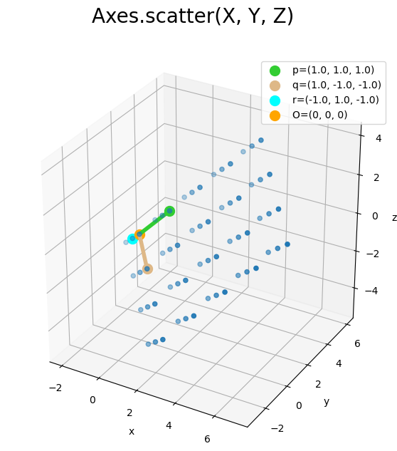
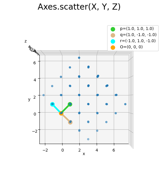
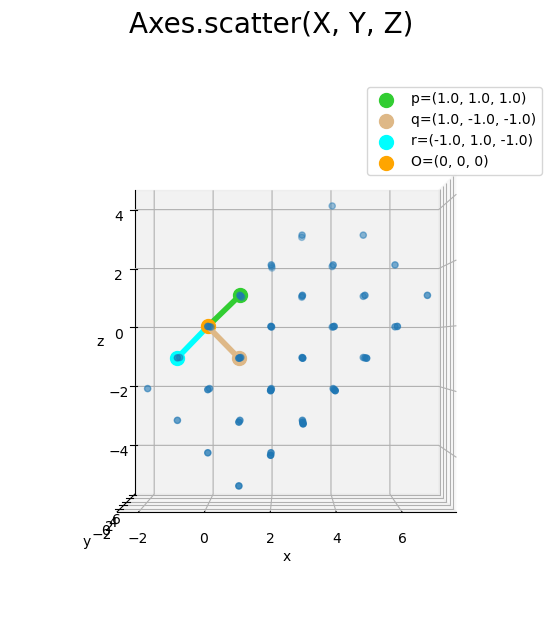
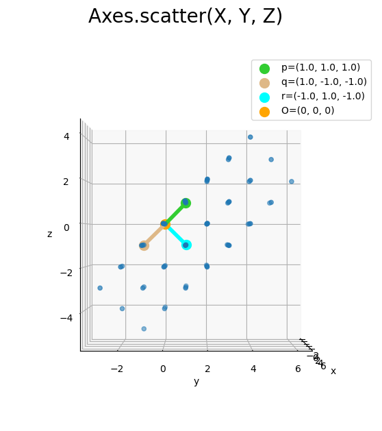
対角線方向にそれぞれ等間隔の点が平行六面体に並びます。面ごとに見ると平行四辺形に並びます。傾きは基準となる点p, q, r、間隔と個数は係数a, b, cによって決まります。
原点(オレンジ色の点)からx軸方向にp[0], q[0], r[0]、y軸方向にp[1], q[1], r[1]、z軸方向にp[2], q[2], r[2]移動した点が点p(黄緑色の点)・点q(ベージュ色の点)・点r(水色の点)です。
X, Y, Zの1つ目の次元(0番目の軸)に関して、for文で繰り返し平面を描画します。
# 平面を作図
fig, ax = plt.subplots(figsize=(7, 7), facecolor='white',
                       subplot_kw={'projection': '3d'})
ax.scatter(X, Y, Z) # 格子点
ax.quiver(0, 0, 0, p[0], p[1], p[2],
          color='limegreen', linewidth=4, arrow_length_ratio=0.0) # pに関する直線
ax.quiver(0, 0, 0, q[0], q[1], q[2],
          color='burlywood', linewidth=4, arrow_length_ratio=0.0) # qに関する直線
ax.quiver(0, 0, 0, r[0], r[1], r[2],
          color='aqua', linewidth=4, arrow_length_ratio=0.0) # rに関する直線
ax.scatter(p[0], p[1], p[2],
           color='limegreen', s=100,
           label='p=('+', '.join(map(str, p.round(2)))+')') # 点p
ax.scatter(q[0], q[1], q[2],
           color='burlywood', s=100,
           label='q=('+', '.join(map(str, q.round(2)))+')') # 点q
ax.scatter(r[0], r[1], r[2],
           color='aqua', s=100,
           label='r=('+', '.join(map(str, r.round(2)))+')') # 点r
ax.scatter(0, 0, 0,
           color='orange', s=100, label='O=(0, 0, 0)') # 原点
for i in range(len(b)):
    ax.plot_wireframe(X[i], Y[i], Z[i], alpha=0.5) # p,rに関する平面
ax.set_xlabel('x')
ax.set_ylabel('y')
ax.set_zlabel('z')
fig.suptitle('Axes.plot_wireframe(X[i], Y[i], Z[i])', fontsize=20)
ax.legend()
ax.set_aspect('equal')
#ax.view_init(elev=0, azim=270) # xz面
plt.show()
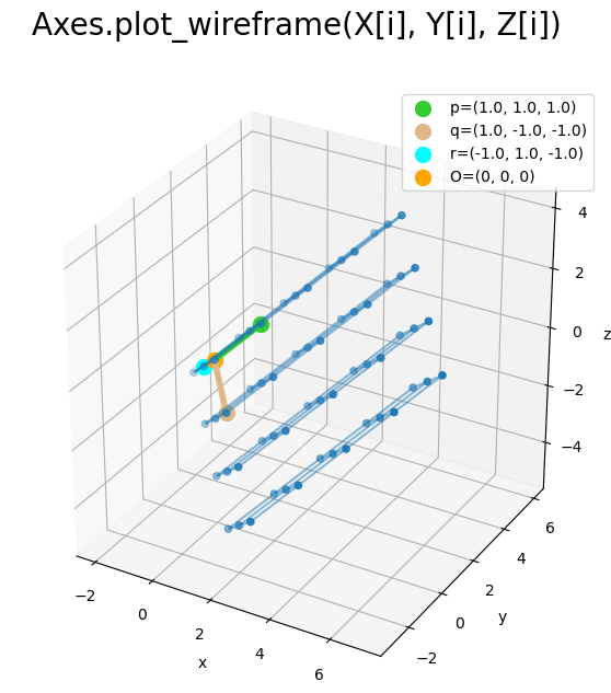
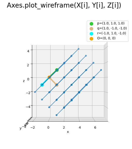
bの要素数(X, Y, Zの0番目の軸の要素数len(X)やX.shape[0])に応じて、原点と点p, rを通る平面と平行な平面です。
同様に、X, Y, Zの2つ目の次元(1番目の軸)に関して平面を描画します。
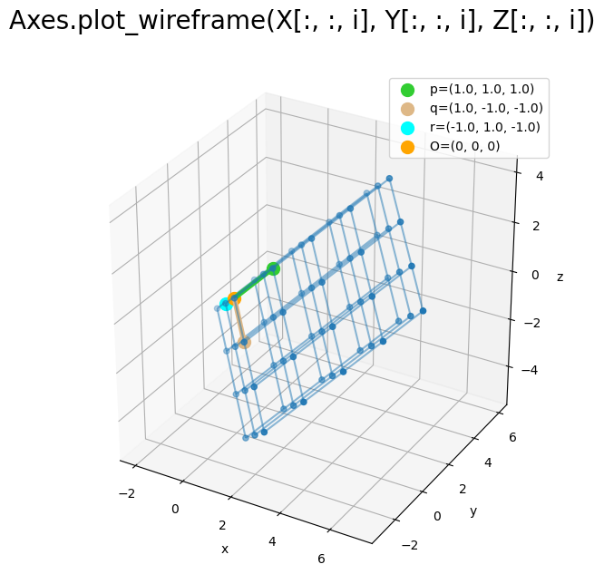
# 平面を作図
fig, ax = plt.subplots(figsize=(7, 7), facecolor='white',
                       subplot_kw={'projection': '3d'})
ax.scatter(X, Y, Z) # 格子点
ax.quiver(0, 0, 0, p[0], p[1], p[2],
          color='limegreen', linewidth=4, arrow_length_ratio=0.0) # pに関する直線
ax.quiver(0, 0, 0, q[0], q[1], q[2],
          color='burlywood', linewidth=4, arrow_length_ratio=0.0) # qに関する直線
ax.quiver(0, 0, 0, r[0], r[1], r[2],
          color='aqua', linewidth=4, arrow_length_ratio=0.0) # rに関する直線
ax.scatter(p[0], p[1], p[2],
           color='limegreen', s=100,
           label='p=('+', '.join(map(str, p.round(2)))+')') # 点p
ax.scatter(q[0], q[1], q[2],
           color='burlywood', s=100,
           label='q=('+', '.join(map(str, q.round(2)))+')') # 点q
ax.scatter(r[0], r[1], r[2],
           color='aqua', s=100,
           label='r=('+', '.join(map(str, r.round(2)))+')') # 点r
ax.scatter(0, 0, 0,
           color='orange', s=100, label='O=(0, 0, 0)') # 原点
for i in range(len(a)):
    ax.plot_wireframe(X[:, i], Y[:, i], Z[:, i], alpha=0.5) # q,rに関する平面
ax.set_xlabel('x')
ax.set_ylabel('y')
ax.set_zlabel('z')
fig.suptitle('Axes.plot_wireframe(X[:, i], Y[:, i], Z[:, i])', fontsize=20)
ax.legend()
ax.set_aspect('equal')
#ax.view_init(elev=90, azim=270) # xy面
plt.show()
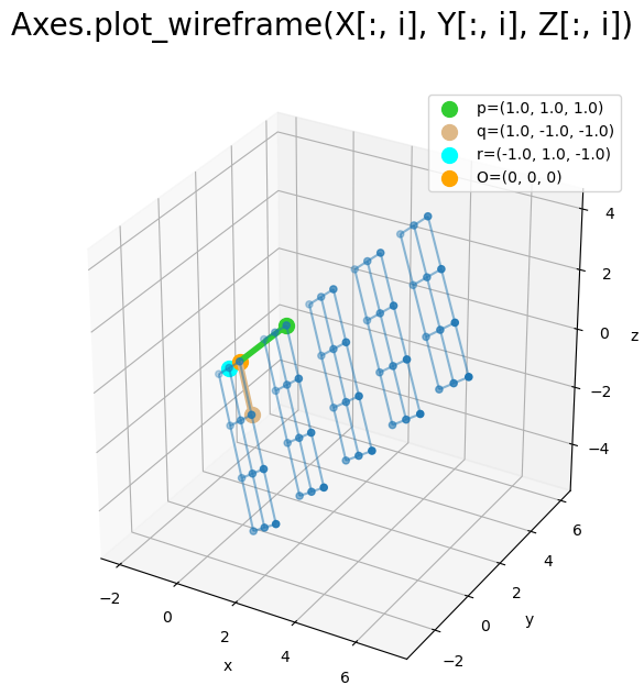
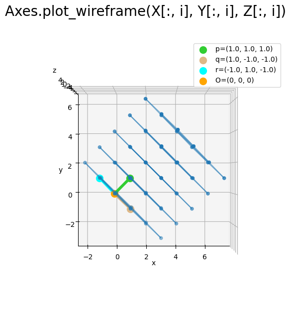
aの要素数(X, Y, Zの1番目の軸の要素数len(X[0])やX.shape[1])に応じて、原点と点q, rを通る平面と平行な平面です。
X, Y, Zの3つ目の次元(2番目の軸)に関して平面を描画します。
# 平面を作図
fig, ax = plt.subplots(figsize=(7, 7), facecolor='white',
                       subplot_kw={'projection': '3d'})
ax.scatter(X, Y, Z) # 格子点
ax.quiver(0, 0, 0, p[0], p[1], p[2],
          color='limegreen', linewidth=4, arrow_length_ratio=0.0) # pに関する直線
ax.quiver(0, 0, 0, q[0], q[1], q[2],
          color='burlywood', linewidth=4, arrow_length_ratio=0.0) # qに関する直線
ax.quiver(0, 0, 0, r[0], r[1], r[2],
          color='aqua', linewidth=4, arrow_length_ratio=0.0) # rに関する直線
ax.scatter(p[0], p[1], p[2],
           color='limegreen', s=100,
           label='p=('+', '.join(map(str, p.round(2)))+')') # 点p
ax.scatter(q[0], q[1], q[2],
           color='burlywood', s=100,
           label='q=('+', '.join(map(str, q.round(2)))+')') # 点q
ax.scatter(r[0], r[1], r[2],
           color='aqua', s=100,
           label='r=('+', '.join(map(str, r.round(2)))+')') # 点r
ax.scatter(0, 0, 0,
           color='orange', s=100, label='O=(0, 0, 0)') # 原点
for i in range(len(c)):
    ax.plot_wireframe(X[:, :, i], Y[:, :, i], Z[:, :, i], alpha=0.5) # p,qに関する平面
ax.set_xlabel('x')
ax.set_ylabel('y')
ax.set_zlabel('z')
fig.suptitle('Axes.plot_wireframe(X[:, :, i], Y[:, :, i], Z[:, :, i])', fontsize=20)
ax.legend()
ax.set_aspect('equal')
#ax.view_init(elev=0, azim=0) # yz面
plt.show()
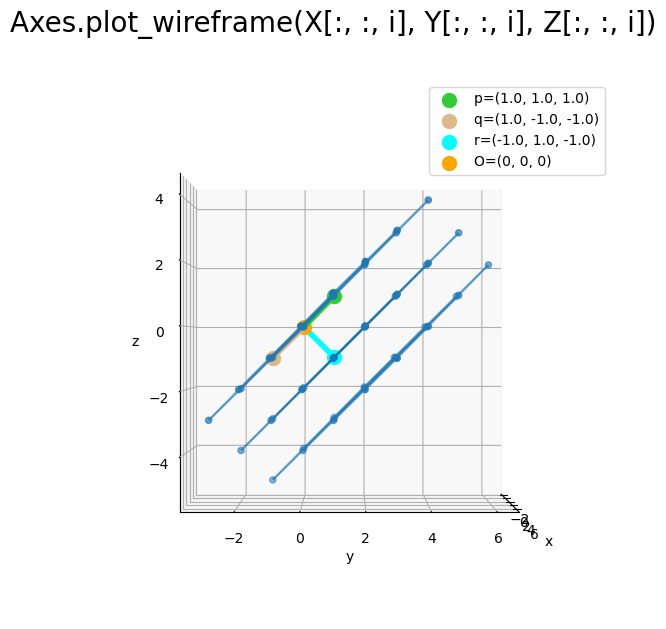
cの要素数(X, Y, Zの2つ目の軸の要素数len(X[0, 0])やX.shape[2])に応じて、原点と点p, qを通る平面と平行な平面です。
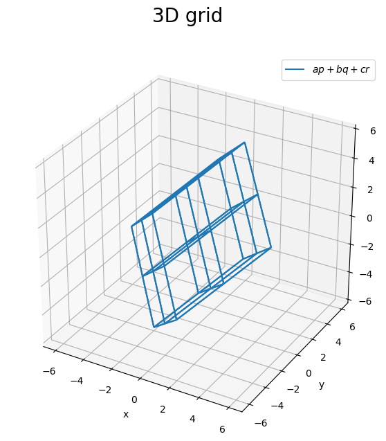
X, Y, Zの全ての次元に関してそれぞれ平面を描画します。
# 3D格子を作図
fig, ax = plt.subplots(figsize=(7, 7), facecolor='white',
                       subplot_kw={'projection': '3d'})
ax.scatter(X, Y, Z) # 格子点
ax.quiver(0, 0, 0, p[0], p[1], p[2],
          color='limegreen', linewidth=4, arrow_length_ratio=0.0) # pに関する直線
ax.quiver(0, 0, 0, q[0], q[1], q[2],
          color='burlywood', linewidth=4, arrow_length_ratio=0.0) # qに関する直線
ax.quiver(0, 0, 0, r[0], r[1], r[2],
          color='aqua', linewidth=4, arrow_length_ratio=0.0) # rに関する直線
ax.scatter(p[0], p[1], p[2],
           color='limegreen', s=100,
           label='p=('+', '.join(map(str, p.round(2)))+')') # 点p
ax.scatter(q[0], q[1], q[2],
           color='burlywood', s=100,
           label='q=('+', '.join(map(str, q.round(2)))+')') # 点q
ax.scatter(r[0], r[1], r[2],
           color='aqua', s=100,
           label='r=('+', '.join(map(str, r.round(2)))+')') # 点r
ax.scatter(0, 0, 0,
           color='orange', s=100, label='O=(0, 0, 0)') # 原点
for i in range(len(b)):
    #  凡例用に1つだけラベルを設定
    if i == 0:
        label_text = '$a p + b q + c r$'
    else:
        label_text = ''
    ax.plot_wireframe(X[i], Y[i], Z[i], alpha=0.5, label=label_text) # p,rに関する平面
for i in range(len(a)):
    ax.plot_wireframe(X[:, i], Y[:, i], Z[:, i], alpha=0.5) # q,rに関する平面
for i in range(len(c)):
    ax.plot_wireframe(X[:, :, i], Y[:, :, i], Z[:, :, i], alpha=0.5) # p,qに関する平面
ax.set_xlabel('x')
ax.set_ylabel('y')
ax.set_zlabel('z')
fig.suptitle('3D grid', fontsize=20)
ax.legend()
ax.set_aspect('equal')
#ax.view_init(elev=90, azim=270) # xy面
#ax.view_init(elev=0, azim=270) # xz面
#ax.view_init(elev=0, azim=0) # yz面
plt.show()
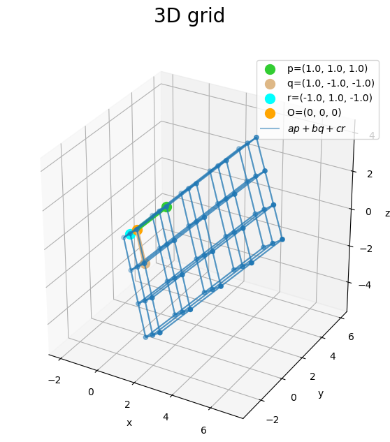
3方向の平面を組み合わせることで、3次元格子を描画できました。
原点とp, q, rそれぞれを結ぶ直線と平行な直線で立体が構成されるので、2方向の面を組み合わせれば、3次元格子を描画できます。
凡例を1つだけ表示するために、1つ目の平面の描画時のみlabel引数に文字列を指定します。if文を使って、初回(iが0のとき)以外は空の文字列''を指定します。
グラフを回転させて確認します。
・作図コード(クリックで展開)
# フレーム数を指定
frame_num = 60

# 水平方向の角度として利用する値を作成
h_n = np.linspace(start=0.0, stop=360.0, num=frame_num+1)[:frame_num]

# グラフオブジェクトを初期化
fig, ax = plt.subplots(figsize=(7, 7), facecolor='white',
                       subplot_kw={'projection': '3d'})
fig.suptitle('3D grid', fontsize=20)

# 作図処理を関数として定義
def update(i):

    # 前フレームのグラフを初期化
    plt.cla()

    # i番目の角度を取得
    h = h_n[i]

    # 3D格子を作図
    ax.scatter(X, Y, Z) # 格子点
    ax.quiver(0, 0, 0, p[0], p[1], p[2],
              color='limegreen', linewidth=4, arrow_length_ratio=0.0) # pに関する直線
    ax.quiver(0, 0, 0, q[0], q[1], q[2],
              color='burlywood', linewidth=4, arrow_length_ratio=0.0) # qに関する直線
    ax.quiver(0, 0, 0, r[0], r[1], r[2],
              color='aqua', linewidth=4, arrow_length_ratio=0.0) # rに関する直線
    ax.scatter(p[0], p[1], p[2],
               color='limegreen', s=100,
               label='p=('+', '.join(map(str, p))+')') # 点p
    ax.scatter(q[0], q[1], q[2],
               color='burlywood', s=100,
               label='q=('+', '.join(map(str, q))+')') # 点q
    ax.scatter(r[0], r[1], r[2],
               color='aqua', s=100,
               label='r=('+', '.join(map(str, r))+')') # 点r
    ax.scatter(0, 0, 0,
               color='orange', s=100, label='O=(0, 0, 0)') # 原点
    for i in range(len(b)):
        # 凡例用に1つだけラベルを設定
        label_text = '$a p + b q + c r$' if i == 0 else ''
        ax.plot_wireframe(X[i], Y[i], Z[i], alpha=0.5, label=label_text) # p,rに関する平面
    for i in range(len(a)):
        ax.plot_wireframe(X[:, i], Y[:, i], Z[:, i], alpha=0.5) # q,rに関する平面
    for i in range(len(c)):
        ax.plot_wireframe(X[:, :, i], Y[:, :, i], Z[:, :, i], alpha=0.5) # p,qに関する平面
    ax.set_xlabel('x')
    ax.set_ylabel('y')
    ax.set_zlabel('z')
    ax.legend(loc='upper left', prop={'size': 8})
    ax.set_aspect('equal')
    ax.view_init(elev=30, azim=h) # 表示角度

# gif画像を作成
ani = FuncAnimation(fig=fig, func=update, frames=frame_num, interval=100)

# gif画像を保存
ani.save('solid360_3d.gif')
作図処理をupdate()として定義して、FuncAnimation()でgif画像を作成します。
if文を1行処理する記法を使っています。
基準となる3点の値を変化させたアニメーションを作成します。
・作図コード(クリックで展開)
# フレーム数を指定
frame_num = 60

# 固定する点の座標を指定
p = np.array([1.0, 1.0, 1.0])
q = np.array([1.0, -1.0, -1.0])

# 変化する点の座標用の値(ラジアン)を作成
t_n = np.linspace(start=0.0, stop=2.0*np.pi, num=frame_num+1)[:frame_num]
u_n = np.linspace(start=1.0/3.0*np.pi, stop=1.0/3.0*np.pi, num=frame_num+1)[:frame_num]

# グラフオブジェクトを初期化
fig, ax = plt.subplots(figsize=(7, 7), facecolor='white',
                       subplot_kw={'projection': '3d'})
fig.suptitle('3D grid', fontsize=20)

# 作図処理を関数として定義
def update(i):

    # 前フレームのグラフを初期化
    plt.cla()

    # i番目の値を取得
    t = t_n[i]
    u = u_n[i]

    # 変化する点の座標を作成
    r = np.array([np.sin(t)*np.cos(u), np.sin(t)*np.sin(u), np.cos(t)])

    # 立体の座標を計算
    X = A * p[0] + B * q[0] + C * r[0]
    Y = A * p[1] + B * q[1] + C * r[1]
    Z = A * p[2] + B * q[2] + C * r[2]

    # 3D格子を作図
    ax.scatter(X, Y, Z) # 格子点
    ax.quiver(0, 0, 0, p[0], p[1], p[2],
              color='limegreen', linewidth=4, arrow_length_ratio=0.0) # pに関する直線
    ax.quiver(0, 0, 0, q[0], q[1], q[2],
              color='burlywood', linewidth=4, arrow_length_ratio=0.0) # qに関する直線
    ax.quiver(0, 0, 0, r[0], r[1], r[2],
              color='aqua', linewidth=4, arrow_length_ratio=0.0) # rに関する直線
    ax.scatter(p[0], p[1], p[2],
               color='limegreen', s=100,
               label='p=('+', '.join(map(str, p.round(2)))+')') # 点p
    ax.scatter(q[0], q[1], q[2],
               color='burlywood', s=100,
               label='q=('+', '.join(map(str, q.round(2)))+')') # 点q
    ax.scatter(r[0], r[1], r[2],
               color='aqua', s=100,
               label='r=('+', '.join(map(str, r.round(2)))+')') # 点r
    ax.scatter(0, 0, 0,
               color='orange', s=100, label='O=(0, 0, 0)') # 原点
    for i in range(len(b)):
        # 凡例用に1つだけラベルを設定
        label_text = '$a p + b q + c r$' if i == 0 else ''
        ax.plot_wireframe(X[i], Y[i], Z[i], alpha=0.5, label=label_text) # p,rに関する平面
    for i in range(len(a)):
        ax.plot_wireframe(X[:, i], Y[:, i], Z[:, i], alpha=0.5) # q,rに関する平面
    for i in range(len(c)):
        ax.plot_wireframe(X[:, :, i], Y[:, :, i], Z[:, :, i], alpha=0.5) # p,qに関する平面
    ax.set_xlabel('x')
    ax.set_ylabel('y')
    ax.set_zlabel('z')
    ax.legend(loc='upper left', prop={'size': 8})
    ax.set_xlim(left=-1.0, right=8.0)
    ax.set_ylim(bottom=-6.0, top=6.0)
    ax.set_zlim(bottom=-5.0, top=6.0)
    ax.set_aspect('equal')

# gif画像を作成
ani = FuncAnimation(fig=fig, func=update, frames=frame_num, interval=100)

# gif画像を保存
ani.save('solid_3d.gif')
この例では、点rが単位球面上を移動し、それに応じて格子の形(平行六面体の立体)が変化します。
3次元配列X, Y, Zの全ての次元を(1次元配列x, y, zを)同じ要素数にしておくと、1つのfor文で処理できます。
# 点の座標を指定
p = np.array([1.0, 1.0, 1.0])
q = np.array([1.0, -1.0, -1.0])
r = np.array([-1.0, 1.0, -1.0])

# 立体用の係数を指定
a = np.arange(start=-2.0, stop=2.1, step=2.0)
print(a.shape)

# 係数の格子点を作成
A, B, C = np.meshgrid(a, a, a)
print(A.shape)
print(B.shape)
print(C.shape)

# 立体の座標を計算
X = A * p[0] + B * q[0] + C * r[0]
Y = A * p[1] + B * q[1] + C * r[1]
Z = A * p[2] + B * q[2] + C * r[2]

# 3D格子を作図
fig, ax = plt.subplots(figsize=(7, 7), facecolor='white',
                       subplot_kw={'projection': '3d'})
for i in range(len(X)):
    #  凡例用に1つだけラベルを設定
    label_text = '$a p + b q + c r$' if i == 0 else ''
    ax.plot_wireframe(X[i], Y[i], Z[i], label=label_text) # p,rに関する平面
    ax.plot_wireframe(X[:, i], Y[:, i], Z[:, i]) # q,rに関する平面
    ax.plot_wireframe(X[:, :, i], Y[:, :, i], Z[:, :, i]) # p,qに関する平面
ax.set_xlabel('x')
ax.set_ylabel('y')
ax.set_zlabel('z')
fig.suptitle('3D grid', fontsize=20)
ax.legend()
ax.set_aspect('equal')
#ax.view_init(elev=90, azim=270) # xy面
#ax.view_init(elev=0, azim=270) # xz面
#ax.view_init(elev=0, azim=0) # yz面
plt.show()
(3,)
(3, 3, 3)
(3, 3, 3)
(3, 3, 3)
以上で、傾いた3次元の格子のグラフを作成します。次は、円のグラフを作成します。
おわりに
これで格子編(なんだそりゃ)が完成です。次は円編です。
【次の内容】