はじめに
『ゼロから作るDeep Learning 4 ――強化学習編』の独学時のまとめノートです。初学者の補助となるようにゼロつくシリーズの4巻の内容に解説を加えていきます。本と一緒に読んでください。
この記事は、7.1.3節の内容です。DeZeroを利用して勾配降下法を実装します。
【前節の内容】
【他の記事一覧】
【この記事の内容】
7.1.3 最適化
DeZeroライブラリを使って、勾配降下法によりローゼンブロック関数の最小値を求めます。DeZeroフレームワークについては「『ゼロから作るDeep Learning 3』の学習ノート:記事一覧 - からっぽのしょこ」を参照してください。
利用するラブライブを読み込みます。
# ライブラリを読み込み
import numpy as np
from dezero import Variable
import dezero.functions as F

# 追加ライブラリ
import matplotlib.pyplot as plt
from matplotlib.colors import LogNorm
from matplotlib.animation import FuncAnimation
更新推移をアニメーションで確認するのにmatplotlibのモジュールを利用します。不要であれば省略してください。
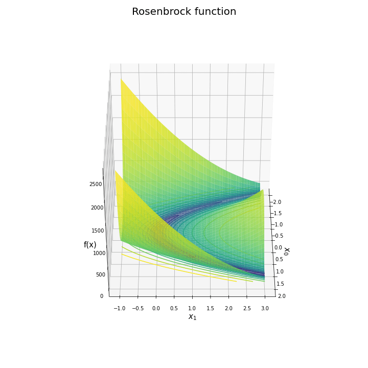
ローゼンブロック関数
まずは、ローゼンブロック関数を可視化します。ローゼンブロック関数の作図については「ステップ28:ローゼンブロック関数の可視化【ゼロつく3のノート(メモ)】 - からっぽのしょこ」を参照してください。
ローゼンブロック関数の計算を関数として定義します。
# ローゼンブロック関数を作成
def rosenbrock(x0, x1):
    # ローゼンブロック関数を計算
    y = 100 * (x1 - x0**2)**2 + (x0 - 1)**2
    return y
ローゼンブロック関数は、次の式で定義されます。
作図用の値を作成します。
# x軸・y軸の値を作成
x0_vals = np.linspace(-2.0, 2.0, num=250)
x1_vals = np.linspace(-1.0, 3.0, num=250)

# 格子点を作成
x0_grid, x1_grid = np.meshgrid(x0_vals, x1_vals)

# z軸の値を計算
y_grid = rosenbrock(x0_grid, x1_grid)

# 対数をとった最小値・最大値を取得
y_log10_min = np.floor(np.log10(y_grid.min()) - 1.0)
y_log10_max = np.ceil(np.log10(y_grid.max()) + 1.0)

# 等高線を引く値を作成
lev_log10 = np.linspace(y_log10_min, y_log10_max, num=45)[25:35]
levs = np.power(10, lev_log10)
x軸($x_0$)とy軸($x_1$)の値x*_valsを指定して、np.meshgrid()で格子点x*_gridに変換して、z軸($y$)の値y_gridを計算します。
対数をとったy_gridの最小値と最大値を使って、等高線を引く値levsを作成します。
ローゼンブロック関数の等高線図を作成します。
# ローゼンブロック関数の等高線図を作成
plt.figure(figsize=(9, 8), facecolor='white')
cnt = plt.contour(x0_grid, x1_grid, y_grid,
                  norm=LogNorm(), levels=levs) # 等高線
plt.scatter(1.0, 1.0,
            marker='*', s=500, c='blue') # 最小値
plt.xlabel('$x_0$', fontsize=15)
plt.ylabel('$x_1$', fontsize=15)
plt.suptitle('Rosenbrock function', fontsize=20)
plt.title('$\mathrm{argmin}_x f(x) = (1, 1)$', loc='left')
plt.colorbar(cnt, label='f(x)')
plt.grid()
plt.axis('equal')
plt.show()

等高線図をplt.contour()で描画します。
最小値の点を星印で示します。
続いて、3Dグラフを作成します。
# ローゼンブロック関数の曲面図を作成
fig = plt.figure(figsize=(10, 10), facecolor='white')
ax = fig.add_subplot(projection='3d') # 3D用の設定
ax.contour(x0_grid, x1_grid, y_grid,
           norm=LogNorm(), levels=levs, offset=0.0) # 等高線
ax.plot_surface(x0_grid, x1_grid, y_grid,
                norm=LogNorm(), cmap='viridis', alpha=0.8) # 曲面
ax.scatter(1.0, 1.0, rosenbrock(1.0, 1.0),
           marker='*', s=500, c='red') # 最小値
ax.set_xlabel('$x_0$', fontsize=15)
ax.set_ylabel('$x_1$', fontsize=15)
ax.set_zlabel('f(x)', fontsize=15)
fig.suptitle('Rosenbrock function', fontsize=20)
ax.set_box_aspect(aspect=(1, 1, 1))
plt.show()

曲面図をax.plot_surface()で描画します。
水平方向に一回転するアニメーションで確認します。
・作図コード(クリックで展開)
# 水平方向の角度として利用する値を指定
h_vals = np.arange(0.0, 360.0, step=5.0)

# フレーム数を設定
frame_num = len(h_vals)

# 図を初期化
fig = plt.figure(figsize=(10, 10), facecolor='white')
ax = fig.add_subplot(projection='3d') # 3D用の設定
fig.suptitle('Rosenbrock function', fontsize=20)

# 作図処理を関数として定義
def update(i):
    # 前フレームのグラフを初期化
    plt.cla()

    # i番目の角度を取得
    h = h_vals[i]

    # ローゼンブロック関数の曲面図を描画
    ax.contour(x0_grid, x1_grid, y_grid,
               norm=LogNorm(), levels=levs, offset=0.0) # 等高線
    ax.plot_surface(x0_grid, x1_grid, y_grid,
                    norm=LogNorm(), cmap='viridis', alpha=0.8) # 曲面
    ax.scatter(1.0, 1.0, rosenbrock(1.0, 1.0),
               marker='*', s=500, c='red') # 最小値
    ax.set_xlabel('$x_0$', fontsize=15)
    ax.set_ylabel('$x_1$', fontsize=15)
    ax.set_zlabel('f(x)', fontsize=15)
    ax.set_box_aspect(aspect=(1, 1, 1))
    ax.view_init(elev=40, azim=h) # 表示角度

# gif画像を作成
ani = FuncAnimation(fig=fig, func=update, frames=frame_num, interval=100)

# gif画像を保存
ani.save('rosenbrock.gif')
作図処理を関数update()として定義して、FuncAnimation()でアニメーション(gif画像)を作成します。
z軸の表示範囲を設定する場合は、次のように処理します。
# z軸の最大値を指定
z_max = 900

# 表示範囲外をマスク
y_mask_grid = np.ma.masked_where(y_grid >= z_max, y_grid)

# ローゼンブロック関数の曲面図を作成
fig = plt.figure(figsize=(10, 9), facecolor='white')
ax = fig.add_subplot(projection='3d') # 3D用の設定
ax.contour(x0_grid, x1_grid, y_grid,
           norm=LogNorm(), levels=levs, offset=0.0) # 等高線
ax.plot_surface(x0_grid, x1_grid, y_mask_grid,
                norm=LogNorm(), cmap='viridis', alpha=0.8) # 曲面
ax.scatter(1.0, 1.0, rosenbrock(1.0, 1.0),
           marker='*', s=500, c='red') # 最小値
ax.set_xlabel('$x_0$', fontsize=15)
ax.set_ylabel('$x_1$', fontsize=15)
ax.set_zlabel('f(x)', fontsize=15)
fig.suptitle('Rosenbrock function', fontsize=20)
ax.set_box_aspect(aspect=(1, 1, 0.5))
ax.set_zlim(-z_max*0.1, z_max)
plt.show()

曲面図の最小値・最大値は、ax.set_zlim()で制御できないので、表示範囲外の値をnp.ma.masked_where()でマスクして描画します。
ここまでは、ローゼンブロック関数を確認しました。
勾配降下法
次は、勾配降下法による学習を実装します。勾配降下法については「6.1.2:SGD【ゼロつく1のノート(実装)】 - からっぽのしょこ」や「ステップ29:勾配降下法とニュートン法の比較【ゼロつく3のノート(数学)】 - からっぽのしょこ」を参照してください。
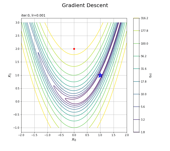
初期値を指定して、勾配降下法によりローゼンブロック関数が最小となる変数を求めます。
# 初期値を指定
x0 = Variable(np.array(0.0))
x1 = Variable(np.array(2.0))

# 学習率を指定
lr = 0.001

# 試行回数を指定
iters = 10000

# 推移の確認用のリストを初期化
trace_x0 = [x0.data.copy()]
trace_x1 = [x1.data.copy()]

# 繰り返し学習
for i in range(iters):
    # ローゼンブロック関数(順伝播)を計算
    y = rosenbrock(x0, x1)

    # 勾配を初期化
    x0.cleargrad()
    x1.cleargrad()

    # 勾配(逆伝播)を計算
    y.backward()

    # 勾配降下法により値を更新
    x0.data -= lr * x0.grad.data
    x1.data -= lr * x1.grad.data

    # 更新値を保存
    trace_x0.append(x0.data.copy())
    trace_x1.append(x1.data.copy())

    # 一定回数ごとに値を表示
    if (i+1) % 500 == 0:
        print(
            'iter ' + str(i+1) +
            ': x=(' + str(np.round(x0.data, 3)) +
            ', ' + str(np.round(x1.data, 3)) + ')'
        )
iter 500: x=(0.529, 0.277)
iter 1000: x=(0.684, 0.466)
iter 1500: x=(0.77, 0.592)
iter 2000: x=(0.826, 0.682)
iter 2500: x=(0.866, 0.749)
iter 3000: x=(0.895, 0.8)
iter 3500: x=(0.917, 0.84)
iter 4000: x=(0.933, 0.871)
iter 4500: x=(0.947, 0.896)
iter 5000: x=(0.957, 0.916)
iter 5500: x=(0.965, 0.932)
iter 6000: x=(0.972, 0.944)
iter 6500: x=(0.977, 0.955)
iter 7000: x=(0.981, 0.963)
iter 7500: x=(0.985, 0.97)
iter 8000: x=(0.988, 0.975)
iter 8500: x=(0.99, 0.98)
iter 9000: x=(0.992, 0.984)
iter 9500: x=(0.993, 0.987)
iter 10000: x=(0.994, 0.989)
処理の内容については本を参照してください。
ローゼンブロック関数の等高線図に、更新値の推移を重ねて描画します。
# 等高線図を作成
plt.figure(figsize=(9, 8), facecolor='white')
cnt = plt.contour(x0_grid, x1_grid, y_grid,
                  norm=LogNorm(), levels=levs) # 等高線
plt.scatter(1.0, 1.0,
            marker='*', s=500, c='blue') # 最小値
plt.plot(trace_x0, trace_x1,
         c='orange', marker='o', mfc='red', mec='red') # 更新値の推移
plt.xlabel('$x_0$', fontsize=15)
plt.ylabel('$x_1$', fontsize=15)
plt.suptitle('Gradient Descent', fontsize=20)
plt.title('iter:'+str(iters) + ', lr='+str(lr), loc='left')
plt.colorbar(cnt, label='f(x)')
plt.grid()
plt.axis('equal')
plt.show()

最小値の点(星印)まで辿り着いているのが分かります。
同様に、曲面図に更新値の推移を重ねて描画します。
# 更新値のz軸の値を計算
trace_y = rosenbrock(np.array(trace_x0), np.array(trace_x1))

# ローゼンブロック関数の曲面図を作成
fig = plt.figure(figsize=(10, 9), facecolor='white')
ax = fig.add_subplot(projection='3d') # 3D用の設定
ax.contour(x0_grid, x1_grid, y_grid,
           norm=LogNorm(), levels=levs, offset=0.0, zorder=0) # 等高線
ax.plot_surface(x0_grid, x1_grid, y_mask_grid,
                norm=LogNorm(), cmap='viridis', alpha=0.8, zorder=1) # 曲面
ax.scatter(1.0, 1.0, rosenbrock(1.0, 1.0),
           marker='*', s=500, c='red') # 最小値
ax.plot(trace_x0, trace_x1, trace_y,
        c='orange', marker='o', mfc='red', mec='red', zorder=15) # 更新値の推移
ax.set_xlabel('$x_0$', fontsize=15)
ax.set_ylabel('$x_1$', fontsize=15)
ax.set_zlabel('f(x)', fontsize=15)
ax.set_title('iter:'+str(iters) + ', lr='+str(lr), loc='left')
fig.suptitle('Gradient descent', fontsize=20)
ax.set_box_aspect(aspect=(1, 1, 0.5))
ax.set_zlim(-z_max*0.1, z_max)
ax.view_init(elev=30, azim=240)
plt.show()

更新値trace_*ごとにz軸の値を計算して描画します。
更新値の推移をアニメーションで確認します。
・作図コード(クリックで展開)
# フレーム数を指定
frame_num = 101

# 図を初期化
fig =plt.figure(figsize=(9, 8), facecolor='white')
fig.suptitle('Gradient descent', fontsize=20)

# カラーバー
tmp = plt.contour(x0_grid, x1_grid, y_grid,
                  norm=LogNorm(), levels=levs) # カラーバー用のダミー
fig.colorbar(tmp, label='f(x)')

# 作図処理を関数として定義
def update(i):
    # 前フレームのグラフを初期化
    plt.cla()

    # 等高線図と更新値を描画
    cnt = plt.contour(x0_grid, x1_grid, y_grid,
                      norm=LogNorm(), levels=levs) # 等高線
    plt.scatter(1.0, 1.0,
                marker='*', s=500, c='blue') # 最小値
    plt.plot(trace_x0[:(i+1)], trace_x1[:(i+1)],
             c='orange', marker='o', mfc='red', mec='red') # 更新値の推移
    plt.xlabel('$x_0$', fontsize=15)
    plt.ylabel('$x_1$', fontsize=15)
    plt.suptitle('Gradient Descent', fontsize=20)
    plt.title('iter:'+str(i) + ', lr='+str(lr), loc='left')
    plt.grid()
    plt.axis('equal')

# gif画像を作成
ani = FuncAnimation(fig=fig, func=update, frames=frame_num, interval=100)

# gif画像を保存
ani.save('GradientDescent_cnt.gif')
# フレーム数を指定
frame_num = 101

# 図を初期化
fig = plt.figure(figsize=(10, 9), facecolor='white')
ax = fig.add_subplot(projection='3d') # 3D用の設定
fig.suptitle('Gradient descent', fontsize=20)

# 作図処理を関数として定義
def update(i):
    # 前フレームのグラフを初期化
    plt.cla()

    # i回目までの更新値のz軸の値を計算
    trace_y = rosenbrock(np.array(trace_x0[:(i+1)]), np.array(trace_x1[:(i+1)]))

    # 曲面図と更新値を描画
    ax.contour(x0_grid, x1_grid, y_grid,
               norm=LogNorm(), levels=levs, offset=0.0, zorder=0) # 等高線
    ax.plot_surface(x0_grid, x1_grid, y_mask_grid,
                    norm=LogNorm(), cmap='viridis', alpha=0.8, zorder=1) # 曲面
    ax.scatter(1.0, 1.0, rosenbrock(1.0, 1.0),
               marker='*', s=500, c='red') # 最小値
    ax.plot(trace_x0[:(i+1)], trace_x1[:(i+1)], trace_y,
            c='orange', marker='o', mfc='red', mec='red', zorder=15) # 更新値の推移
    ax.set_xlabel('$x_0$', fontsize=15)
    ax.set_ylabel('$x_1$', fontsize=15)
    ax.set_zlabel('f(x)', fontsize=15)
    ax.set_title('iter:'+str(i) + ', lr='+str(lr), loc='left')
    ax.set_box_aspect(aspect=(1, 1, 0.5))
    ax.set_zlim(-z_max*0.1, z_max)
    ax.view_init(elev=30, azim=240) # 表示角度

# gif画像を作成
ani = FuncAnimation(fig=fig, func=update, frames=frame_num, interval=100)

# gif画像を保存
ani.save('GradientDescent_srf.gif')
フレームごとにtrace_*からi番目までの値を取り出して点を描画する処理を関数update()として定義して、FuncAnimation()でアニメーション(gif画像)を作成します。

変数の更新値の推移をグラフで確認します。
# 更新値の推移を作図
plt.figure(figsize=(8, 6), facecolor='white')
plt.plot(np.arange(iters+1), trace_x0, label='$x_0$')
plt.plot(np.arange(iters+1), trace_x1, label='$x_1$')
plt.xlabel('iteration')
plt.ylabel('x')
plt.suptitle('$x = (x_0, x_1)$', fontsize=20)
plt.legend()
plt.grid()
plt.show()

最小値となる点$(1, 1)$に近付いているのが分かります。
この節では、DeZeroの使い方と勾配降下法を実装しました。次節は、勾配降下法を用いて線形回帰を実装します。
参考文献

おわりに
7章の1つ目の記事です。1巻と3巻の復習ですね。7章を読み終わった時点だとどちらも読んでなくても大丈夫そうですが、その後はどうでしょう。
zorder引数の仕様がよく分からない。
【次節の内容】