はじめに
『スタンフォード ベクトル・行列からはじめる最適化数学』の学習ノートです。
本の内容に関して「Pythonを使って再現」や「数式の行間埋め」によって理解を目指します。本と一緒に読んでください。
この記事は1.2節「ベクトルの和」の内容です。
ベクトルの差を可視化します。
【前の内容】
【他の内容】
【今回の内容】
ベクトルの差の可視化
2つのベクトルの差をグラフで確認します。
利用するライブラリを読み込みます。
# 利用ライブラリ
import numpy as np
import matplotlib.pyplot as plt
from matplotlib.animation import FuncAnimation
2次元の場合
まずは、2次元空間(平面)上でベクトルの差を可視化します。
2つの2次元ベクトルを指定します。
# ベクトルを指定
a = np.array([5.0, 1.0])
b = np.array([-1.0, 3.0])
を
a、を
bとして値を指定します。ただし、Pythonでは0からインデックスが割り当てられるので、の値は
a[0]に対応します。
a-b
2次元空間(平面)上に3つのベクトル描画します。
# 作図用の値を設定
x_min = np.floor(np.min([0.0, a[0], b[0], -b[0]])) - 1
x_max = np.ceil(np.max([0.0, a[0], b[0], -b[0]])) + 1
y_min = np.floor(np.min([0.0, a[1], b[1], -b[1]])) - 1
y_max = np.ceil(np.max([0.0, a[1], b[1], -b[1]])) + 1

# (原点からの)2Dベクトルを作図
fig, ax = plt.subplots(figsize=(6, 6), facecolor='white')
ax.quiver(0, 0, *a, color='red', angles='xy', scale_units='xy', scale=1) # ベクトルa
ax.quiver(0, 0, *b, color='turquoise', angles='xy', scale_units='xy', scale=1) # ベクトルb
ax.quiver(0, 0, *-b, color='blue', angles='xy', scale_units='xy', scale=1) # ベクトル-b
ax.annotate(xy=0.5*a, text='a', size=15, ha='center', va='top') # ベクトルaラベル
ax.annotate(xy=0.5*b, text='b', size=15, ha='right', va='center') # ベクトルbラベル
ax.annotate(xy=-0.5*b, text='-b', size=15, ha='right', va='center') # ベクトル-bラベル
ax.set_xticks(ticks=np.arange(x_min, x_max+1))
ax.set_yticks(ticks=np.arange(y_min, y_max+1))
ax.grid()
ax.set_xlabel('x')
ax.set_ylabel('y')
ax.set_title('a=('+', '.join(map(str, a))+'), ' +
             'b=('+', '.join(map(str, b))+')', loc='left')
fig.suptitle('vector a, b, -b', fontsize=20)
ax.set_aspect('equal')
plt.show()
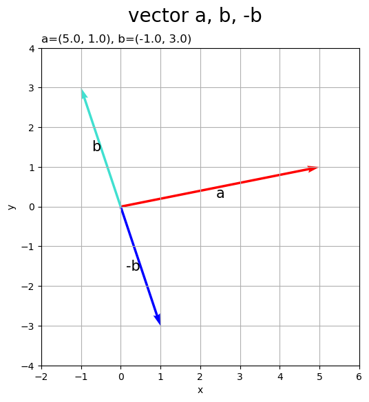
ベクトルのグラフを
axes.quiver()で描画します。第1・2引数に始点の座標、第3・4引数にベクトルのサイズ(変化量)を指定します。この例では、原点を始点とします。
配列a, bの前に*を付けてアンパック(展開)して指定しています。
は、
を反対に向けたベクトルです。ベクトルの-1倍については「【Python】1.3:ベクトルのスカラー倍の可視化【『スタンフォード線形代数入門』のノート】 - からっぽのしょこ」を参照してください。
のベクトルを描画します。
# 作図用の値を設定
x_min = np.floor(np.min([0.0, a[0], b[0]])) - 1
x_max = np.ceil(np.max([0.0, a[0], b[0]])) + 1
y_min = np.floor(np.min([0.0, a[1], b[1]])) - 1
y_max = np.ceil(np.max([0.0, a[1], b[1]])) + 1

# 2Dベクトル差を作図
fig, ax = plt.subplots(figsize=(6, 4), facecolor='white')
ax.quiver(0, 0, *a, color='red', angles='xy', scale_units='xy', scale=1) # ベクトルa
ax.quiver(*b, *-b, color='blue', angles='xy', scale_units='xy', scale=1) # ベクトル-b
ax.quiver(*b, *a-b, color='purple', angles='xy', scale_units='xy', scale=1) # ベクトルa-b
ax.annotate(xy=0.5*a, text='a', size=15, ha='center', va='top') # ベクトルaラベル
ax.annotate(xy=0.5*b, text='-b', size=15, ha='right', va='center') # ベクトル-bラベル
ax.annotate(xy=0.5*(a+b), text='a-b', size=15, ha='left', va='bottom') # ベクトルa-bラベル
ax.set_xticks(ticks=np.arange(x_min, x_max+1))
ax.set_yticks(ticks=np.arange(y_min, y_max+1))
ax.grid()
ax.set_xlabel('x')
ax.set_ylabel('y')
ax.set_title('a=('+', '.join(map(str, a))+'), ' +
             'b=('+', '.join(map(str, b))+')', loc='left')
fig.suptitle('vector a-b', fontsize=20)
ax.set_aspect('equal')
plt.show()

ベクトルの始点を点
にすると、「【Python】1.2:ベクトルの和の可視化【『スタンフォード線形代数入門』のノート】 - からっぽのしょこ」のときと同様にして、ベクトル
と
の関係を示せます。
原点と点を重ねて描画します。
# 2Dベクトル差を作図
fig, ax = plt.subplots(figsize=(6, 4), facecolor='white')
ax.quiver(0, 0, *a, color='red', angles='xy', scale_units='xy', scale=1, label='a') # ベクトルa
ax.quiver(*b, *-b, color='blue', angles='xy', scale_units='xy', scale=1, label='-b') # ベクトル-b
ax.quiver(*b, *a-b, color='purple', angles='xy', scale_units='xy', scale=1, label='a-b') # ベクトルa-b
ax.scatter(0, 0, c='orange', s=100) # 原点
ax.scatter(*a, c='red', s=100) # 点a
ax.scatter(*b, c='blue', s=100) # 点b
ax.annotate(xy=[0, 0], text='O', size=15, ha='right', va='top') # 原点ラベル
ax.annotate(xy=a, text='a', size=15, ha='left', va='top') # 点aラベル
ax.annotate(xy=b, text='b', size=15, ha='right', va='bottom') # 点bラベル
ax.set_xticks(ticks=np.arange(x_min, x_max+1))
ax.set_yticks(ticks=np.arange(y_min, y_max+1))
ax.grid()
ax.set_xlabel('x')
ax.set_ylabel('y')
ax.set_title('a=('+', '.join(map(str, a))+'), ' +
             'b=('+', '.join(map(str, b))+')', loc='left')
fig.suptitle('point a, b', fontsize=20)
ax.legend()
ax.set_aspect('equal')
plt.show()
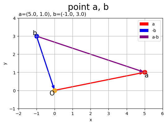
ベクトルは、点
から点
の移動を表すのが分かります。
ベクトルの値を変化させたアニメーションを作成します。
・作図コード(クリックで展開)
# フレーム数を設定
frame_num = 51

# 各次元の要素として利用する値を指定
a_vals = np.array(
    [np.linspace(start=-6.0, stop=6.0, num=frame_num),
     np.linspace(start=0.0, stop=10.0, num=frame_num)]
).T
b_vals = np.array(
    [np.linspace(start=-1.0, stop=-1.0, num=frame_num),
     np.linspace(start=3.0, stop=3.0, num=frame_num)]
).T

# 作図用の値を設定
x_min = np.floor(np.min([0.0, *a_vals[:, 0], *b_vals[:, 0], *a_vals[:, 0]+b_vals[:,0]])) - 1
x_max = np.ceil(np.max([0.0, *a_vals[:, 0], *b_vals[:, 0], *a_vals[:, 0]+b_vals[:, 0]])) + 1
y_min = np.floor(np.min([0.0, *a_vals[:, 1], *b_vals[:, 1], *a_vals[:, 1]+b_vals[:, 1]])) - 1
y_max = np.ceil(np.max([0.0, *a_vals[:, 1], *b_vals[:, 1], *a_vals[:, 1]+b_vals[:, 1]])) + 1

# 作図用のオブジェクトを初期化
fig, ax = plt.subplots(figsize=(8, 8), facecolor='white')
fig.suptitle('vector a-b', fontsize=20)

# 作図処理を関数として定義
def update(i):

    # 前フレームのグラフを初期化
    plt.cla()

    # i番目のベクトルを作成
    a = a_vals[i]
    b = b_vals[i]

    # 2Dベクトル差を作図
    ax.quiver(0, 0, *a, color='red', angles='xy', scale_units='xy', scale=1) # ベクトルa
    ax.quiver(*b, *-b, color='blue', angles='xy', scale_units='xy', scale=1) # ベクトル-b
    ax.quiver(*b, *a-b, color='purple', angles='xy', scale_units='xy', scale=1) # ベクトルa-b
    ax.annotate(xy=0.5*a, text='a', size=15, ha='center', va='top') # ベクトルaラベル
    ax.annotate(xy=0.5*b, text='-b', size=15, ha='right', va='center') # ベクトル-bラベル
    ax.annotate(xy=0.5*(a+b), text='a-b', size=15, ha='right', va='bottom') # ベクトルa-bラベル
    ax.set_xticks(ticks=np.arange(x_min, x_max+1))
    ax.set_yticks(ticks=np.arange(y_min, y_max+1))
    ax.grid()
    ax.set_xlabel('x')
    ax.set_ylabel('y')
    ax.set_title('a=('+', '.join(map(str, a.round(2)))+'), ' +
                 'b=('+', '.join(map(str, b.round(2)))+')', loc='left')
    ax.set_aspect('equal')

# gif画像を作成
ani = FuncAnimation(fig=fig, func=update, frames=frame_num, interval=100)

# gif画像を保存
ani.save('diff_ab_vector_2d.gif')
作図処理をupdate()として定義して、FuncAnimation()でgif画像を作成します。
b-a
同様に、平面上に3つのベクトル描画します。
# 作図用の値を設定
x_min = np.floor(np.min([0.0, a[0], -a[0], b[0]])) - 1
x_max = np.ceil(np.max([0.0, a[0], -a[0], b[0]])) + 1
y_min = np.floor(np.min([0.0, a[1], -a[1], b[1]])) - 1
y_max = np.ceil(np.max([0.0, a[1], -a[1], b[1]])) + 1

# ベクトルを作図
fig, ax = plt.subplots(figsize=(6, 4), facecolor='white')
ax.quiver(0, 0, *a, color='hotpink', angles='xy', scale_units='xy', scale=1) # ベクトルa
ax.quiver(0, 0, *-a, color='red', angles='xy', scale_units='xy', scale=1) # ベクトル-a
ax.quiver(0, 0, *b, color='blue', angles='xy', scale_units='xy', scale=1) # ベクトル-b
ax.annotate(xy=0.5*a, text='-a', size=15, ha='center', va='top') # ベクトルaラベル
ax.annotate(xy=-0.5*a, text='-a', size=15, ha='center', va='top') # ベクトル-aラベル
ax.annotate(xy=0.5*b, text='b', size=15, ha='right', va='center') # ベクトル-bラベル
ax.set_xticks(ticks=np.arange(x_min, x_max+1))
ax.set_yticks(ticks=np.arange(y_min, y_max+1))
ax.grid()
ax.set_xlabel('x')
ax.set_ylabel('y')
ax.set_title('a=('+', '.join(map(str, a))+'), ' +
             'b=('+', '.join(map(str, b))+')', loc='left')
fig.suptitle('vector a, -a, b', fontsize=20)
ax.set_aspect('equal')
plt.show()
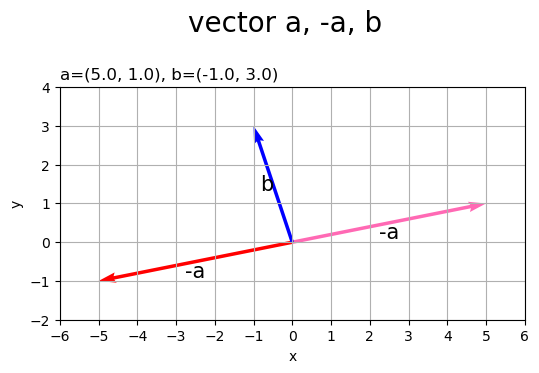
は、
を反対に向けたベクトルです。
のベクトルを描画します。
# 作図用の値を設定
x_min = np.floor(np.min([0.0, a[0], b[0]])) - 1
x_max = np.ceil(np.max([0.0, a[0], b[0]])) + 1
y_min = np.floor(np.min([0.0, a[1], b[1]])) - 1
y_max = np.ceil(np.max([0.0, a[1], b[1]])) + 1

# ベクトルを作図
fig, ax = plt.subplots(figsize=(6, 4), facecolor='white')
ax.quiver(*a, *-a, color='red', angles='xy', scale_units='xy', scale=1) # ベクトル-a
ax.quiver(0, 0, *b, color='blue', angles='xy', scale_units='xy', scale=1) # ベクトルb
ax.quiver(*a, *b-a, color='purple', angles='xy', scale_units='xy', scale=1) # ベクトルb-a
ax.annotate(xy=0.5*a, text='-a', size=15, ha='center', va='top') # ベクトル-aラベル
ax.annotate(xy=0.5*b, text='b', size=15, ha='right', va='center') # ベクトルbラベル
ax.annotate(xy=0.5*(a+b), text='b-a', size=15, ha='left', va='bottom') # ベクトルb-aラベル
ax.set_xticks(ticks=np.arange(x_min, x_max+1))
ax.set_yticks(ticks=np.arange(y_min, y_max+1))
ax.grid()
ax.set_xlabel('x')
ax.set_ylabel('y')
ax.set_title('a=('+', '.join(map(str, a))+'), ' +
             'b=('+', '.join(map(str, b))+')', loc='left')
fig.suptitle('vector b-a', fontsize=20)
ax.set_aspect('equal')
plt.show()
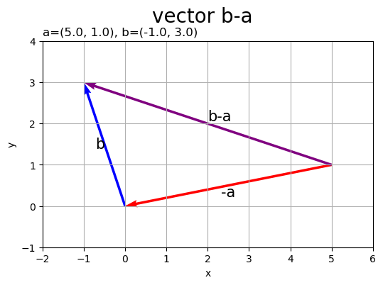
ベクトルの始点を点
にすると、ベクトル
と
の関係を示せます。
は、
を反対に向けたベクトルであり、
なのが分かります。
原点と点を重ねて描画します。
# 2Dベクトル差を作図
fig, ax = plt.subplots(figsize=(6, 4), facecolor='white')
ax.quiver(*a, *-a, color='red', angles='xy', scale_units='xy', scale=1, label='-a') # ベクトル-a
ax.quiver(0, 0, *b, color='blue', angles='xy', scale_units='xy', scale=1, label='b') # ベクトルb
ax.quiver(*a, *b-a, color='purple', angles='xy', scale_units='xy', scale=1, label='b-a') # ベクトルb-a
ax.scatter(0, 0, c='orange', s=100) # 原点
ax.scatter(*a, c='red', s=100) # 点a
ax.scatter(*b, c='blue', s=100) # 点b
ax.annotate(xy=[0, 0], text='O', size=15, ha='right', va='top') # 原点ラベル
ax.annotate(xy=a, text='a', size=15, ha='left', va='top') # 点aラベル
ax.annotate(xy=b, text='b', size=15, ha='right', va='bottom') # 点bラベル
ax.set_xticks(ticks=np.arange(x_min, x_max+1))
ax.set_yticks(ticks=np.arange(y_min, y_max+1))
ax.grid()
ax.set_xlabel('x')
ax.set_ylabel('y')
ax.set_title('a=('+', '.join(map(str, a))+'), ' +
             'b=('+', '.join(map(str, b))+')', loc='left')
fig.suptitle('point a, b', fontsize=20)
ax.legend()
ax.set_aspect('equal')
plt.show()
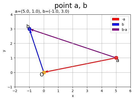
ベクトルは、点
から点
の移動を表すのが分かります。
ベクトルの値を変化させたアニメーションを作成します。
・作図コード(クリックで展開)
# フレーム数を設定
frame_num = 51

# 各次元の要素として利用する値を指定
a_vals = np.array(
    [np.linspace(start=-6.0, stop=6.0, num=frame_num),
     np.linspace(start=0.0, stop=10.0, num=frame_num)]
).T
b_vals = np.array(
    [np.linspace(start=-1.0, stop=-1.0, num=frame_num),
     np.linspace(start=3.0, stop=3.0, num=frame_num)]
).T

# 作図用の値を設定
x_min = np.floor(np.min([0.0, *a_vals[:, 0], *b_vals[:, 0], *a_vals[:, 0]+b_vals[:,0]])) - 1
x_max = np.ceil(np.max([0.0, *a_vals[:, 0], *b_vals[:, 0], *a_vals[:, 0]+b_vals[:, 0]])) + 1
y_min = np.floor(np.min([0.0, *a_vals[:, 1], *b_vals[:, 1], *a_vals[:, 1]+b_vals[:, 1]])) - 1
y_max = np.ceil(np.max([0.0, *a_vals[:, 1], *b_vals[:, 1], *a_vals[:, 1]+b_vals[:, 1]])) + 1

# 作図用のオブジェクトを初期化
fig, ax = plt.subplots(figsize=(8, 8), facecolor='white')
fig.suptitle('vector b-a', fontsize=20)

# 作図処理を関数として定義
def update(i):

    # 前フレームのグラフを初期化
    plt.cla()

    # i番目のベクトルを作成
    a = a_vals[i]
    b = b_vals[i]

    # 2Dベクトル差を作図
    ax.quiver(*a, *-a, color='red', angles='xy', scale_units='xy', scale=1) # ベクトル-a
    ax.quiver(0, 0, *b, color='blue', angles='xy', scale_units='xy', scale=1) # ベクトルb
    ax.quiver(*a, *b-a, color='purple', angles='xy', scale_units='xy', scale=1) # ベクトルb-a
    ax.annotate(xy=0.5*a, text='-a', size=15, ha='center', va='top') # ベクトル-aラベル
    ax.annotate(xy=0.5*b, text='b', size=15, ha='right', va='center') # ベクトルbラベル
    ax.annotate(xy=0.5*(a+b), text='b-a', size=15, ha='right', va='bottom') # ベクトルb-aラベル
    ax.set_xticks(ticks=np.arange(x_min, x_max+1))
    ax.set_yticks(ticks=np.arange(y_min, y_max+1))
    ax.grid()
    ax.set_xlabel('x')
    ax.set_ylabel('y')
    ax.set_title('a=('+', '.join(map(str, a.round(2)))+'), ' +
                 'b=('+', '.join(map(str, b.round(2)))+')', loc='left')
    ax.set_aspect('equal')

# gif画像を作成
ani = FuncAnimation(fig=fig, func=update, frames=frame_num, interval=100)

# gif画像を保存
ani.save('diff_ba_vector_2d.gif')
3次元の場合
続いて、3次元空間上でベクトルの差を可視化します。
3次元ベクトルを指定します。
# ベクトルを指定
a = np.array([5.0, 1.0, 3.0])
b = np.array([-1.0, 3.0, 2.0])
を
a、を
bとして値を指定します。
a-b
3次元空間上に3つのベクトルを描画します。
# 作図用の値を設定
x_min = np.floor(np.min([0.0, a[0], b[0], -b[0]])) - 1
x_max = np.ceil(np.max([0.0, a[0], b[0], -b[0]])) + 1
y_min = np.floor(np.min([0.0, a[1], b[1], -b[1]])) - 1
y_max = np.ceil(np.max([0.0, a[1], b[1], -b[1]])) + 1
z_min = np.floor(np.min([0.0, a[2], b[2], -b[2]])) - 1
z_max = np.ceil(np.max([0.0, a[2], b[2], -b[2]])) + 1

# (原点からの)3Dベクトルを作図
fig, ax = plt.subplots(figsize=(8, 8), subplot_kw={'projection': '3d'}, facecolor='white')
ax.quiver(0, 0, 0, *a, color='red', arrow_length_ratio=0.1) # ベクトルa
ax.quiver(0, 0, 0, *b, color='turquoise', arrow_length_ratio=0.1) # ベクトルb
ax.quiver(0, 0, 0, *-b, color='blue', arrow_length_ratio=0.1) # ベクトル-b
ax.text(*0.5*a, s='a', size=15, ha='center', va='top') # ベクトルaラベル
ax.text(*0.5*b, s='b', size=15, ha='right', va='center') # ベクトルbラベル
ax.text(*-0.5*b, s='-b', size=15, ha='right', va='center') # ベクトル-bラベル
ax.quiver([0, a[0], b[0], -b[0]], [0, a[1], b[1], -b[1]], [z_min, z_min, z_min, z_min],
          [0, 0, 0, 0], [0, 0, 0, 0], [-z_min, a[2]-z_min, b[2]-z_min, -b[2]-z_min],
          color='gray', arrow_length_ratio=0, linestyle=':') # 補助線
ax.set_xticks(ticks=np.arange(x_min, x_max+1))
ax.set_yticks(ticks=np.arange(y_min, y_max+1))
ax.set_zticks(ticks=np.arange(z_min, z_max+1))
ax.set_zlim(z_min, z_max)
ax.set_xlabel('x')
ax.set_ylabel('y')
ax.set_zlabel('z')
ax.set_title('a=('+', '.join(map(str, a))+'), ' +
             'b=('+', '.join(map(str, b))+')', loc='left')
fig.suptitle('vector a, b, -b', fontsize=20)
ax.set_aspect('equal')
plt.show()
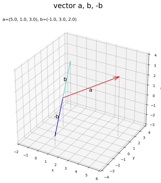
axes.quiver()の第1・2・3引数に始点の座標、第4・5・6引数にベクトルのサイズを指定します。この例では、原点を始点とします。
のベクトルを描画します。
# 作図用の値を設定
x_min = np.floor(np.min([0.0, a[0], b[0]])) - 1
x_max = np.ceil(np.max([0.0, a[0], b[0]])) + 1
y_min = np.floor(np.min([0.0, a[1], b[1]])) - 1
y_max = np.ceil(np.max([0.0, a[1], b[1]])) + 1
z_min = np.floor(np.min([0.0, a[2], b[2]])) - 1
z_max = np.ceil(np.max([0.0, a[2], b[2]])) + 1

# 3Dベクトル和を作図
fig, ax = plt.subplots(figsize=(8, 8), subplot_kw={'projection': '3d'}, facecolor='white')
ax.quiver(0, 0, 0, *a, color='red', arrow_length_ratio=0.1) # ベクトルa
ax.quiver(*b, *-b, color='blue', arrow_length_ratio=0.1) # ベクトル-b
ax.quiver(*b, *a-b, color='purple', arrow_length_ratio=0.1) # ベクトルa-b
ax.text(*0.5*a, s='a', size=15, ha='center', va='top') # ベクトルaラベル
ax.text(*0.5*b, s='-b', size=15, ha='right', va='center') # ベクトル-bラベル
ax.text(*0.5*(a+b), s='a-b', size=15, ha='left', va='bottom') # ベクトルa-bラベル
ax.quiver([0, a[0], b[0]], [0, a[1], b[1]], [z_min, z_min, z_min],
          [0, 0, 0], [0, 0, 0], [-z_min, a[2]-z_min, b[2]-z_min],
          color='gray', arrow_length_ratio=0, linestyle=':') # 補助線
ax.set_xticks(ticks=np.arange(x_min, x_max+1))
ax.set_yticks(ticks=np.arange(y_min, y_max+1))
ax.set_zticks(ticks=np.arange(z_min, z_max+1))
ax.set_zlim(z_min, z_max)
ax.set_xlabel('x')
ax.set_ylabel('y')
ax.set_zlabel('z')
ax.set_title('a=('+', '.join(map(str, a))+'), ' +
             'b=('+', '.join(map(str, b))+')', loc='left')
fig.suptitle('vector a-b', fontsize=20)
ax.set_aspect('equal')
plt.show()
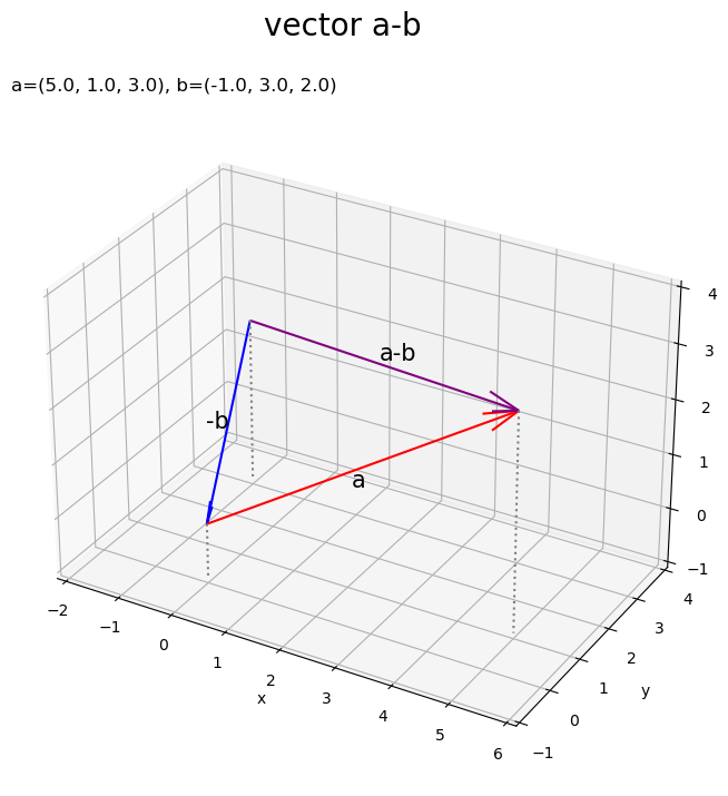
3次元の場合も、と
の和が
になるのが分かります。
原点と点を重ねて描画します。
# 3Dベクトル和を作図
fig, ax = plt.subplots(figsize=(8, 8), subplot_kw={'projection': '3d'}, facecolor='white')
ax.quiver(0, 0, 0, *a, color='red', arrow_length_ratio=0.1, label='a') # ベクトルa
ax.quiver(*b, *-b, color='blue', arrow_length_ratio=0.1, label='-b') # ベクトル-b
ax.quiver(*b, *a-b, color='purple', arrow_length_ratio=0.1, label='a-b') # ベクトルa-b
ax.scatter(0, 0, 0, c='orange', s=100) # 原点
ax.scatter(*a, c='red', s=100) # 点a
ax.scatter(*b, c='blue', s=100) # 点b
ax.text(0, 0, 0, s='O', size=15, ha='center', va='top', zorder=20) # 原点ラベル
ax.text(*a, s='a', size=15, ha='center', va='top', zorder=20) # 点aラベル
ax.text(*b, s='b', size=15, ha='right', va='center', zorder=20) # 点bラベル
ax.quiver([0, a[0], b[0]], [0, a[1], b[1]], [z_min, z_min, z_min],
          [0, 0, 0], [0, 0, 0], [-z_min, a[2]-z_min, b[2]-z_min],
          color='gray', arrow_length_ratio=0, linestyle=':') # 補助線
ax.set_xticks(ticks=np.arange(x_min, x_max+1))
ax.set_yticks(ticks=np.arange(y_min, y_max+1))
ax.set_zticks(ticks=np.arange(z_min, z_max+1))
ax.set_zlim(z_min, z_max)
ax.set_xlabel('x')
ax.set_ylabel('y')
ax.set_zlabel('z')
ax.set_title('a=('+', '.join(map(str, a))+'), ' +
             'b=('+', '.join(map(str, b))+')', loc='left')
fig.suptitle('point a, b', fontsize=20)
ax.legend()
ax.set_aspect('equal')
plt.show()
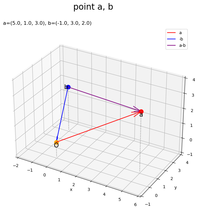
3次元でも、ベクトルが点
から点
の移動を表すのが分かります。
ベクトルの値を変化させたアニメーションを作成します。
・作図コード(クリックで展開)
# フレーム数を設定
frame_num = 51

# 各次元の要素として利用する値を指定
a_vals = np.array(
    [np.linspace(start=-6.0, stop=6.0, num=frame_num),
     np.linspace(start=0.0, stop=10.0, num=frame_num),
     np.linspace(start=-2.0, stop=3.0, num=frame_num)]
).T
b_vals = np.array(
    [np.linspace(start=-1.0, stop=-1.0, num=frame_num),
     np.linspace(start=3.0, stop=3.0, num=frame_num),
     np.linspace(start=2.0, stop=2.0, num=frame_num)]
).T

# 作図用の値を設定
x_min = np.floor(np.min([0.0, *a_vals[:, 0], *b_vals[:, 0]])) - 1
x_max = np.ceil(np.max([0.0, *a_vals[:, 0], *b_vals[:, 0]])) + 1
y_min = np.floor(np.min([0.0, *a_vals[:, 1], *b_vals[:, 1]])) - 1
y_max = np.ceil(np.max([0.0, *a_vals[:, 1], *b_vals[:, 1]])) + 1
z_min = np.floor(np.min([0.0, *a_vals[:, 2], *b_vals[:, 2]])) - 1
z_max = np.ceil(np.max([0.0, *a_vals[:, 2], *b_vals[:, 2]])) + 1

# 作図用のオブジェクトを初期化
fig, ax = plt.subplots(figsize=(8, 8), subplot_kw={'projection': '3d'}, facecolor='white')
fig.suptitle('vector b-a', fontsize=20)

# 作図処理を関数として定義
def update(i):

    # 前フレームのグラフを初期化
    plt.cla()

    # i番目のベクトルを作成
    a = a_vals[i]
    b = b_vals[i]

    # 3Dベクトル和を作図
    ax.quiver(0, 0, 0, *a, color='red', arrow_length_ratio=0.1) # ベクトルa
    ax.quiver(*b, *-b, color='blue', arrow_length_ratio=0.1) # ベクトル-b
    ax.quiver(*b, *a-b, color='purple', arrow_length_ratio=0.1) # ベクトルa-b
    ax.text(*0.5*a, s='a', size=15, ha='center', va='top') # ベクトルaラベル
    ax.text(*0.5*b, s='-b', size=15, ha='right', va='center') # ベクトル-bラベル
    ax.text(*0.5*(a+b), s='a-b', size=15, ha='left', va='bottom') # ベクトルa-bラベル
    ax.quiver([0, a[0], b[0]], [0, a[1], b[1]], [z_min, z_min, z_min],
              [0, 0, 0], [0, 0, 0], [-z_min, a[2]-z_min, b[2]-z_min],
              color='gray', arrow_length_ratio=0, linestyle=':') # 補助線
    ax.set_xticks(ticks=np.arange(x_min, x_max+1))
    ax.set_yticks(ticks=np.arange(y_min, y_max+1))
    ax.set_zticks(ticks=np.arange(z_min, z_max+1))
    ax.set_zlim(z_min, z_max)
    ax.set_xlabel('x')
    ax.set_ylabel('y')
    ax.set_zlabel('z')
    ax.set_title('a=('+', '.join(map(str, a.round(2)))+'), ' +
                 'b=('+', '.join(map(str, b.round(2)))+')', loc='left')
    ax.set_aspect('equal')

# gif画像を作成
ani = FuncAnimation(fig=fig, func=update, frames=frame_num, interval=100)

# gif画像を保存
ani.save('diff_ab_vector_3d.gif')
b-a
同様に、3次元空間上に3つのベクトルを描画します。
# 作図用の値を設定
x_min = np.floor(np.min([0.0, a[0], -a[0], b[0]])) - 1
x_max = np.ceil(np.max([0.0, a[0], -a[0], b[0]])) + 1
y_min = np.floor(np.min([0.0, a[1], -a[1], b[1]])) - 1
y_max = np.ceil(np.max([0.0, a[1], -a[1], b[1]])) + 1
z_min = np.floor(np.min([0.0, a[2], -a[2], b[2]])) - 1
z_max = np.ceil(np.max([0.0, a[2], -a[2], b[2]])) + 1

# (原点からの)3Dベクトルを作図
fig, ax = plt.subplots(figsize=(8, 8), subplot_kw={'projection': '3d'}, facecolor='white')
ax.quiver(0, 0, 0, *a, color='hotpink', arrow_length_ratio=0.1) # ベクトルa
ax.quiver(0, 0, 0, *-a, color='red', arrow_length_ratio=0.1) # ベクトル-a
ax.quiver(0, 0, 0, *b, color='blue', arrow_length_ratio=0.1) # ベクトルb
ax.text(*0.5*a, s='a', size=15, ha='center', va='top') # ベクトルaラベル
ax.text(*-0.5*a, s='-a', size=15, ha='right', va='center') # ベクトル-aラベル
ax.text(*0.5*b, s='b', size=15, ha='right', va='center') # ベクトルbラベル
ax.quiver([0, a[0], -a[0], b[0]], [0, a[1], -a[1], b[1]], [z_min, z_min, z_min, z_min],
          [0, 0, 0, 0], [0, 0, 0, 0], [-z_min, a[2]-z_min, -a[2]-z_min, b[2]-z_min],
          color='gray', arrow_length_ratio=0, linestyle=':') # 補助線
ax.set_xticks(ticks=np.arange(x_min, x_max+1))
ax.set_yticks(ticks=np.arange(y_min, y_max+1))
ax.set_zticks(ticks=np.arange(z_min, z_max+1))
ax.set_zlim(z_min, z_max)
ax.set_xlabel('x')
ax.set_ylabel('y')
ax.set_zlabel('z')
ax.set_title('a=('+', '.join(map(str, a))+'), ' +
             'b=('+', '.join(map(str, b))+')', loc='left')
fig.suptitle('vector a, -a, b', fontsize=20)
ax.set_aspect('equal')
plt.show()
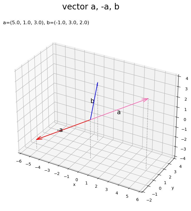
これまでと同様にして作図します。
のベクトルを描画します。
# 作図用の値を設定
x_min = np.floor(np.min([0.0, a[0], b[0]])) - 1
x_max = np.ceil(np.max([0.0, a[0], b[0]])) + 1
y_min = np.floor(np.min([0.0, a[1], b[1]])) - 1
y_max = np.ceil(np.max([0.0, a[1], b[1]])) + 1
z_min = np.floor(np.min([0.0, a[2], b[2]])) - 1
z_max = np.ceil(np.max([0.0, a[2], b[2]])) + 1

# 3Dベクトル差を作図
fig, ax = plt.subplots(figsize=(8, 8), subplot_kw={'projection': '3d'}, facecolor='white')
ax.quiver(*a, *-a, color='red', arrow_length_ratio=0.1) # ベクトル-a
ax.quiver(0, 0, 0, *b, color='blue', arrow_length_ratio=0.1) # ベクトルb
ax.quiver(*a, *b-a, color='purple', arrow_length_ratio=0.1) # ベクトルb-a
ax.text(*0.5*a, s='-a', size=15, ha='center', va='top') # ベクトル-aラベル
ax.text(*0.5*b, s='b', size=15, ha='right', va='center') # ベクトルbラベル
ax.text(*0.5*(a+b), s='b-a', size=15, ha='left', va='bottom') # ベクトルb-aラベル
ax.quiver([0, a[0], b[0]], [0, a[1], b[1]], [z_min, z_min, z_min],
          [0, 0, 0], [0, 0, 0], [-z_min, a[2]-z_min, b[2]-z_min],
          color='gray', arrow_length_ratio=0, linestyle=':') # 補助線
ax.set_xticks(ticks=np.arange(x_min, x_max+1))
ax.set_yticks(ticks=np.arange(y_min, y_max+1))
ax.set_zticks(ticks=np.arange(z_min, z_max+1))
ax.set_zlim(z_min, z_max)
ax.set_xlabel('x')
ax.set_ylabel('y')
ax.set_zlabel('z')
ax.set_title('a=('+', '.join(map(str, a))+'), ' +
             'b=('+', '.join(map(str, b))+')', loc='left')
fig.suptitle('vector b-a', fontsize=20)
ax.set_aspect('equal')
plt.show()
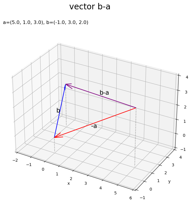
これまでと同様にして作図します。
原点と点を重ねて描画します。
# 3Dベクトル差を作図
fig, ax = plt.subplots(figsize=(8, 8), subplot_kw={'projection': '3d'}, facecolor='white')
ax.quiver(*a, *-a, color='red', arrow_length_ratio=0.1, label='-a') # ベクトル-a
ax.quiver(0, 0, 0, *b, color='blue', arrow_length_ratio=0.1, label='b') # ベクトルb
ax.quiver(*a, *b-a, color='purple', arrow_length_ratio=0.1, label='b-a') # ベクトルb-a
ax.scatter(0, 0, 0, c='orange', s=100) # 原点
ax.scatter(*a, c='red', s=100) # 点a
ax.scatter(*b, c='blue', s=100) # 点b
ax.text(0, 0, 0, s='O', size=15, ha='center', va='top', zorder=20) # 原点ラベル
ax.text(*a, s='a', size=15, ha='center', va='top', zorder=20) # 点aラベル
ax.text(*b, s='b', size=15, ha='right', va='center', zorder=20) # 点bラベル
ax.quiver([0, a[0], b[0]], [0, a[1], b[1]], [z_min, z_min, z_min],
          [0, 0, 0], [0, 0, 0], [-z_min, a[2]-z_min, b[2]-z_min],
          color='gray', arrow_length_ratio=0, linestyle=':') # 補助線
ax.set_xticks(ticks=np.arange(x_min, x_max+1))
ax.set_yticks(ticks=np.arange(y_min, y_max+1))
ax.set_zticks(ticks=np.arange(z_min, z_max+1))
ax.set_zlim(z_min, z_max)
ax.set_xlabel('x')
ax.set_ylabel('y')
ax.set_zlabel('z')
ax.set_title('a=('+', '.join(map(str, a))+'), ' +
             'b=('+', '.join(map(str, b))+')', loc='left')
fig.suptitle('point a, b', fontsize=20)
ax.legend()
ax.set_aspect('equal')
plt.show()
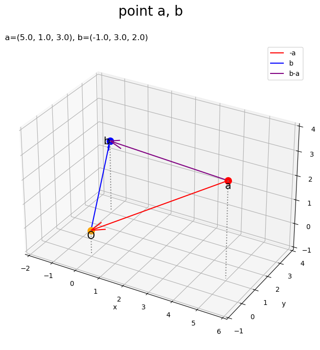
3次元でも、ベクトルが点
から点
の移動を表すのが分かります。
ベクトルの値を変化させたアニメーションを作成します。
・作図コード(クリックで展開)
# フレーム数を設定
frame_num = 51

# 各次元の要素として利用する値を指定
a_vals = np.array(
    [np.linspace(start=-6.0, stop=6.0, num=frame_num),
     np.linspace(start=0.0, stop=10.0, num=frame_num),
     np.linspace(start=-2.0, stop=3.0, num=frame_num)]
).T
b_vals = np.array(
    [np.linspace(start=-1.0, stop=-1.0, num=frame_num),
     np.linspace(start=3.0, stop=3.0, num=frame_num),
     np.linspace(start=2.0, stop=2.0, num=frame_num)]
).T

# 作図用の値を設定
x_min = np.floor(np.min([0.0, *a_vals[:, 0], *b_vals[:, 0]])) - 1
x_max = np.ceil(np.max([0.0, *a_vals[:, 0], *b_vals[:, 0]])) + 1
y_min = np.floor(np.min([0.0, *a_vals[:, 1], *b_vals[:, 1]])) - 1
y_max = np.ceil(np.max([0.0, *a_vals[:, 1], *b_vals[:, 1]])) + 1
z_min = np.floor(np.min([0.0, *a_vals[:, 2], *b_vals[:, 2]])) - 1
z_max = np.ceil(np.max([0.0, *a_vals[:, 2], *b_vals[:, 2]])) + 1

# 作図用のオブジェクトを初期化
fig, ax = plt.subplots(figsize=(8, 8), subplot_kw={'projection': '3d'}, facecolor='white')
fig.suptitle('vector b-a', fontsize=20)

# 作図処理を関数として定義
def update(i):

    # 前フレームのグラフを初期化
    plt.cla()

    # i番目のベクトルを作成
    a = a_vals[i]
    b = b_vals[i]

    # 3Dベクトル差を作図
    ax.quiver(*a, *-a, color='red', arrow_length_ratio=0.1) # ベクトル-a
    ax.quiver(0, 0, 0, *b, color='blue', arrow_length_ratio=0.1) # ベクトルb
    ax.quiver(*a, *b-a, color='purple', arrow_length_ratio=0.1) # ベクトルb-a
    ax.text(*0.5*a, s='-a', size=15, ha='center', va='top') # ベクトル-aラベル
    ax.text(*0.5*b, s='b', size=15, ha='right', va='center') # ベクトルbラベル
    ax.text(*0.5*(a+b), s='b-a', size=15, ha='left', va='bottom') # ベクトルb-aラベル
    ax.quiver([0, a[0], b[0]], [0, a[1], b[1]], [z_min, z_min, z_min],
              [0, 0, 0], [0, 0, 0], [-z_min, a[2]-z_min, b[2]-z_min],
              color='gray', arrow_length_ratio=0, linestyle=':') # 補助線
    ax.set_xticks(ticks=np.arange(x_min, x_max+1))
    ax.set_yticks(ticks=np.arange(y_min, y_max+1))
    ax.set_zticks(ticks=np.arange(z_min, z_max+1))
    ax.set_zlim(z_min, z_max)
    ax.set_xlabel('x')
    ax.set_ylabel('y')
    ax.set_zlabel('z')
    ax.set_title('a=('+', '.join(map(str, a.round(2)))+'), ' +
                 'b=('+', '.join(map(str, b.round(2)))+')', loc='left')
    fig.suptitle('vector b-a', fontsize=20)
    ax.set_aspect('equal')

# gif画像を作成
ani = FuncAnimation(fig=fig, func=update, frames=frame_num, interval=100)

# gif画像を保存
ani.save('diff_ba_vector_3d.gif')
この記事では、ベクトルの差を可視化しました。次の記事では、ベクトルのスカラー倍を可視化します。
参考書籍
- Stephen Boyd・Lieven Vandenberghe(著),玉木 徹(訳)『スタンフォード ベクトル・行列からはじめる最適化数学』講談社サイエンティク,2021年.
おわりに
まだ簡単だなと思いつつも、線形代数を1からちゃんと勉強してないので、知らない事ばっかりでへーとか言いながら書いてます。
【次の内容】