はじめに
円関数(三角関数)の定義や性質、公式などを可視化して理解しようシリーズです。
この記事では、R言語でtangent関数のグラフを作成します。
【前の内容】
【他の記事一覧】
【この記事の内容】
tan関数の定義の可視化
tan関数(正接関数・タンジェント関数・tangent function)の定義をグラフで確認します。tan関数は、円関数(circular functions)・三角関数(trigonometric functions)の1つです。
tan関数の形状(振幅・周期・位相・切片)の変化については各パラメータの記事や「tan関数の波形の可視化」を参照してください。
利用するパッケージを読み込みます。
# 利用パッケージ
library(tidyverse)
この記事では、基本的に パッケージ名::関数名() の記法を使うので、パッケージの読み込みは不要です。ただし、作図コードについてはパッケージ名を省略するので、ggplot2 を読み込む必要があります。
また、ネイティブパイプ演算子 |> を使います。magrittr パッケージのパイプ演算子 %>% に置き換えられますが、その場合は magrittr を読み込む必要があります。
定義式の確認
まずは、tan関数の定義式を確認します。
sin関数については「【R】sin関数の定義の可視化 - からっぽのしょこ」、cos関数については「【R】cos関数の定義の可視化 - からっぽのしょこ」を参照してください。
tan関数は、sin関数とcos関数の商で定義されます。
ただし、 を正負の整数として
のとき、
であり、0除算になるため定義できません。変数
はラジアン(弧度法の角度)、
は円周率です。
曲線の形状
続いて、tan関数の曲線のグラフを作成します。
曲線の作成
・作図コード(クリックで展開)
変数の範囲を指定して、座標計算用のベクトルを作成します。
# 変数(ラジアン)の範囲を指定
theta_vec <- seq(from = -2*pi, to = 2*pi, length.out = 1001)
head(theta_vec)
[1] -6.283185 -6.270619 -6.258053 -6.245486 -6.232920 -6.220353
変数(ラジアン) の範囲を指定して、数値ベクトルを作成します。範囲を
の倍数にすると周期性を確認しやすくなります。円周率
は
pi で扱えます。
曲線の描画用のデータフレームを作成します。
# 閾値を指定
threshold <- 4

# 曲線の座標を作成
curve_df <- tibble::tibble(
  t     = theta_vec,
  tan_t = tan(t),
  sin_t = sin(t),
  cos_t = cos(t)
) |>
  dplyr::mutate(
    tan_t = dplyr::if_else(
      (tan_t >= -threshold & tan_t <= threshold), true = tan_t, false = NA_real_
    )
  ) # 閾値外を欠損値に置換
curve_df
# A tibble: 1,001 × 4
       t    tan_t    sin_t cos_t
   <dbl>    <dbl>    <dbl> <dbl>
 1 -6.28 2.45e-16 2.45e-16 1
 2 -6.27 1.26e- 2 1.26e- 2 1.00
 3 -6.26 2.51e- 2 2.51e- 2 1.00
 4 -6.25 3.77e- 2 3.77e- 2 0.999
 5 -6.23 5.03e- 2 5.02e- 2 0.999
 6 -6.22 6.29e- 2 6.28e- 2 0.998
 7 -6.21 7.55e- 2 7.53e- 2 0.997
 8 -6.20 8.82e- 2 8.79e- 2 0.996
 9 -6.18 1.01e- 1 1.00e- 1 0.995
10 -6.17 1.14e- 1 1.13e- 1 0.994
# ℹ 991 more rows
変数 と関数
の値をデータフレームに格納します。比較用に、
の値も格納しておきます。tan関数は
tan()、sin関数は sin()、cos関数は cos() で計算できます。
ただし範囲によっては、 が発散するので、閾値
threshold を指定しておき、閾値外の値を(数値型の)欠損値 NA に置き換えます。
ラジアン軸目盛の表示用のベクトルを作成します。装飾用の処理です。
# 半周期(範囲π)における目盛数(分母の値)を指定
tick_num <- 2

# 目盛番号(分子の値)の範囲を設定
tick_min <- floor(min(theta_vec) / pi) * tick_num
tick_max <- ceiling(max(theta_vec) / pi) * tick_num

# 目盛番号(分子の値)を作成
tick_vec <- tick_min:tick_max

# 目盛位置を作成
rad_break_vec <- tick_vec/tick_num * pi

# 目盛ラベルを作成
rad_label_vec <- paste(round(rad_break_vec/pi, digits = 2), "* pi")
head(tick_vec); head(rad_break_vec); head(rad_label_vec)
[1] -4 -3 -2 -1  0  1
[1] -6.283185 -4.712389 -3.141593 -1.570796  0.000000  1.570796
[1] "-2 * pi"   "-1.5 * pi" "-1 * pi"   "-0.5 * pi" "0 * pi"    "0.5 * pi"
ラジアン に関する軸目盛ラベルを
を小数にした形で表示することにします。
は半周期(
間隔の範囲)における目盛数、
は(負の数を含む)目盛番号に対応します。
theta_vec の最小値・最大値に対して、 を
について整理した
を計算して、最小番号から最大番号までの整数を作成します。整数にするために、小数部分に関して最小値は
floor() で切り捨て、最大値は ceiling() で切り上げておきます。
作成した目盛番号に対応する目盛位置(ラジアン)を で計算します。
ラベルとして数式(ギリシャ文字や記号)を表示する場合は、expression() の記法を用います。その際に、オブジェクト(プログラム上の変数)を使う場合は、文字列として作成しておき parse() の text 引数に渡します。
漸近線の描画用のベクトルを作成します。
# 漸近線の範囲を設定:(π単位で切り捨て・切り上げ)
theta_lower <- (floor(min(theta_vec) / pi) - 0.5) * pi
theta_upper <- (ceiling(max(theta_vec) / pi) + 0.5) * pi

# 漸近線の位置を作成
asymptote_break_vec <- seq(from = theta_lower, to = theta_upper, by = pi)

# 漸近線のラベルを作成
asymptote_label_vec <- paste(round(asymptote_break_vec/pi, digits = 2), "* pi")
head(asymptote_break_vec); head(asymptote_label_vec)
[1] -7.853982 -4.712389 -1.570796  1.570796  4.712389  7.853982
[1] "-2.5 * pi" "-1.5 * pi" "-0.5 * pi" "0.5 * pi"  "1.5 * pi"  "2.5 * pi"
が発散する位置に漸近線と目盛ラベルを表示することにします。
ラジアン軸目盛と同様に、theta_vec の最小値・最大値を用いて、ラジアン (
は整数)とラベルを作成します。
tan関数のグラフを作成します。
# 関数曲線を作図
ggplot() +
  geom_segment(mapping = aes(x = c(-Inf, 0), y = c(0, -Inf),
                             xend = c(Inf, 0), yend = c(0, Inf)),
               arrow = arrow(length = unit(10, units = "pt"), ends = "last")) + # x・y軸線
  geom_vline(xintercept = asymptote_break_vec,
             linetype = "twodash") + # 漸近線
  geom_line(data = curve_df,
            mapping = aes(x = t, y = tan_t, linetype = "tan"),
            linewidth = 1, na.rm = TRUE) + # tan曲線
  geom_line(data = curve_df,
            mapping = aes(x = t, y = sin_t, linetype = "sin"),
            linewidth = 1) + # sin曲線
  geom_line(data = curve_df,
            mapping = aes(x = t, y = cos_t, linetype = "cos"),
            linewidth = 1) + # cos曲線
  scale_linetype_manual(breaks = c("tan", "sin", "cos"),
                        values = c("solid", "dashed", "dotted"),
                        labels = c(expression(tan~theta), expression(sin~theta), expression(cos~theta)),
                        name = "function") + # 凡例表示用
  scale_x_continuous(breaks = rad_break_vec,
                     labels = parse(text = rad_label_vec),
                     sec.axis = sec_axis(trans = ~.,
                                         breaks = asymptote_break_vec,
                                         labels = parse(text = asymptote_label_vec),
                                         name = "asymptote")) + # ラジアン軸目盛
  guides(linetype = guide_legend(override.aes = list(linewidth = 0.5))) + # 凡例の体裁
  theme(legend.text.align = 1) + # 図の体裁
  coord_fixed(ratio = 1,
              xlim = c(min(theta_vec), max(theta_vec))) + # アスペクト比
  labs(title = "tangent function",
       subtitle = expression(tan~theta == frac(sin~theta, cos~theta)),
       x = expression(theta),
       y = expression(f(theta)))
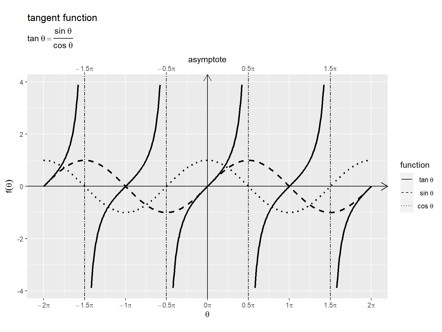
tan曲線を実線、sin曲線を破線、cos曲線を点線で、また漸近線を鎖線で示します。
横軸(変数) はラジアン(弧度法の角度)、
は円周率です。
を整数として、
軸が
の点(
を中心に
間隔)で、
であり
が発散するのを確認できます。また、
軸が
の点(
を中心に
間隔)で、
であり
になります。
次からは、単位円との関係を見ていきます。
単位円の作成
円関数の可視化に利用する単位円(unit circle)のグラフを確認します。
円の作図や度数法と弧度法(角度とラジアン)の関係については「【R】円周の作図 - からっぽのしょこ」を参照してください。
・作図コード(クリックで展開)
単位円の描画用のデータフレームを作成します。
# 円周の座標を作成
circle_df <- tibble::tibble(
  t = seq(from = 0, to = 2*pi, length.out = 361), # 1周期分のラジアン
  r = 1, # 半径
  x = r * cos(t),
  y = r * sin(t)
)
circle_df
# A tibble: 361 × 4
        t     r     x      y
    <dbl> <dbl> <dbl>  <dbl>
 1 0          1 1     0
 2 0.0175     1 1.00  0.0175
 3 0.0349     1 0.999 0.0349
 4 0.0524     1 0.999 0.0523
 5 0.0698     1 0.998 0.0698
 6 0.0873     1 0.996 0.0872
 7 0.105      1 0.995 0.105
 8 0.122      1 0.993 0.122
 9 0.140      1 0.990 0.139
10 0.157      1 0.988 0.156
# ℹ 351 more rows
1周分のラジアン を作成して、単位円の円周のx座標
とy座標
を計算します。
角度(ラジアン)目盛の描画用のデータフレームを作成します。
# 半円(範囲π)における目盛数(分母の値)を指定
tick_num <- 6

# 角度目盛の座標を作成:(補助目盛有り)
d <- 1.1
rad_tick_df <- tibble::tibble(
  # 座標用
  i     = seq(from = 0, to = 2*tick_num-0.5, by = 0.5), # 目盛番号(分子の値)
  t_deg = i/tick_num * 180, # 度数法の角度
  t_rad = i/tick_num * pi,  # 弧度法の角度(ラジアン)
  r     = 1, # 半径
  x     = r * cos(t_rad),
  y     = r * sin(t_rad),
  major_flag = i%%1 == 0, # 主・補助フラグ
  grid       = dplyr::if_else(major_flag, true = "major", false = "minor"), # 目盛カテゴリ
  # ラベル用
  deg_label  = dplyr::if_else(
    major_flag, true = paste0(round(t_deg, digits = 1), "*degree"), false = ""
  ), # 角度ラベル
  rad_label  = dplyr::if_else(
    major_flag, true = paste0("frac(", i, ", ", tick_num, ") ~ pi"), false = ""
  ), # ラジアンラベル
  label_x = d * x,
  label_y = d * y,
  a = t_deg + 90,
  h = 1 - (x * 0.5 + 0.5),
  v = 1 - (y * 0.5 + 0.5),
  tick_mark = dplyr::if_else(major_flag, true = "|", false = "") # 目盛指示線用
)
rad_tick_df
# A tibble: 24 × 16
       i t_deg t_rad     r         x     y major_flag grid  deg_label  rad_label
   <dbl> <dbl> <dbl> <dbl>     <dbl> <dbl> <lgl>      <chr> <chr>      <chr>
 1   0       0 0         1  1   e+ 0 0     TRUE       major "0*degree" "frac(0,…
 2   0.5    15 0.262     1  9.66e- 1 0.259 FALSE      minor ""         ""
 3   1      30 0.524     1  8.66e- 1 0.5   TRUE       major "30*degre… "frac(1,…
 4   1.5    45 0.785     1  7.07e- 1 0.707 FALSE      minor ""         ""
 5   2      60 1.05      1  5   e- 1 0.866 TRUE       major "60*degre… "frac(2,…
 6   2.5    75 1.31      1  2.59e- 1 0.966 FALSE      minor ""         ""
 7   3      90 1.57      1  6.12e-17 1     TRUE       major "90*degre… "frac(3,…
 8   3.5   105 1.83      1 -2.59e- 1 0.966 FALSE      minor ""         ""
 9   4     120 2.09      1 -5   e- 1 0.866 TRUE       major "120*degr… "frac(4,…
10   4.5   135 2.36      1 -7.07e- 1 0.707 FALSE      minor ""         ""
# ℹ 14 more rows
# ℹ 6 more variables: label_x <dbl>, label_y <dbl>, a <dbl>, h <dbl>, v <dbl>,
#   tick_mark <chr>
「曲線の作図」のときと同様に、目盛番号と対応するラジアンを作成して、円周上の座標とラベル用の文字列を作成します。ただし、補助目盛も作成します。主目盛と補助目盛を major_flag 列または grid 列で描き分けます。
目盛ラベル用の座標を label_x, label_y 列として、表示位置を原点からのノルム(半径) d で調整します。
単位円と角度目盛のグラフを作成します。
# グラフサイズを設定
axis_size <- 1.5

# 単位円を作図
ggplot() +
  geom_segment(data = rad_tick_df,
               mapping = aes(x = 0, y = 0, xend = x, yend = y),
               linetype = "dotted") + # 角度目盛線
  geom_text(data = rad_tick_df,
            mapping = aes(x = x, y = y, angle = a, label = tick_mark),
            size = 2) + # 角度目盛指示線
  geom_text(data = rad_tick_df,
            mapping = aes(x = label_x, y = label_y, label = deg_label, hjust = h, vjust = v),
            parse = TRUE) + # 角度目盛ラベル
  geom_path(data = circle_df,
            mapping = aes(x = x, y = y),
            linewidth = 1) + # 円周
  coord_fixed(ratio = 1,
              xlim = c(-axis_size, axis_size),
              ylim = c(-axis_size, axis_size)) + # アスペクト比
  labs(title = "unit circle",
       subtitle = expression(r == 1),
       x = expression(x == r ~ cos~theta),
       y = expression(y == r ~ sin~theta))
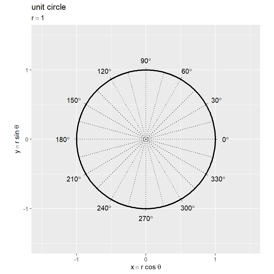
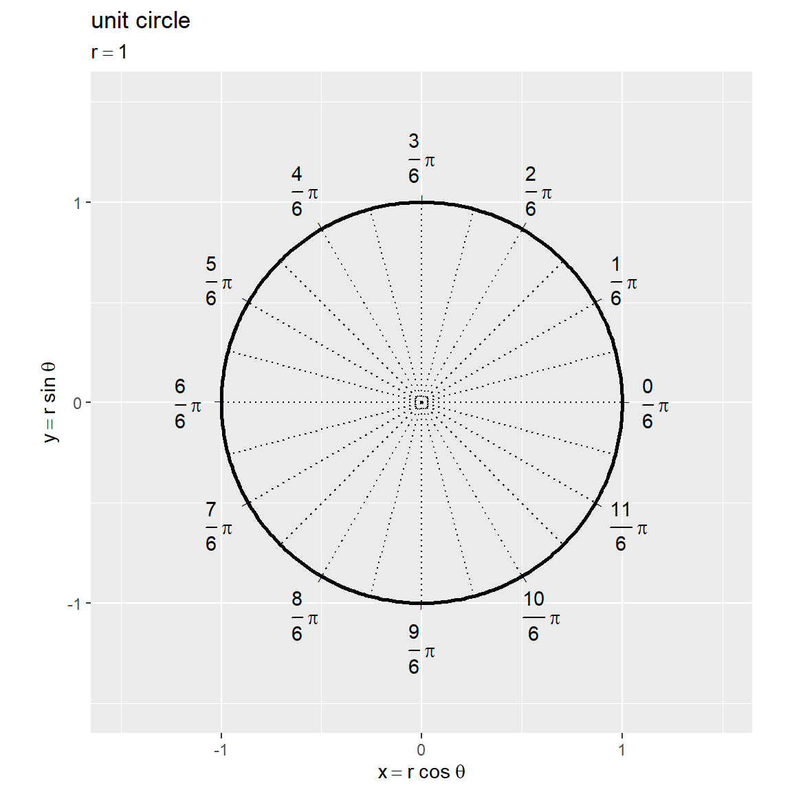
原点を中心とする半径 の円周の座標は
です。半径が
の円を単位円と呼びます。(半径や開始位置に関わらず)偏角が
(度数法だと
)で1周します。
度数法の角度 と弧度法の角度
は
の関係です。
このグラフ上に円関数の値を線分として描画します。
単位円と関数の関係
次は、単位円における偏角(単位円周上の点)と円関数(tan・sin・cos・exsec)の関係を可視化します。
各関数についてはそれぞれの記事を参照してください。
グラフの作成
変数を固定して、単位円におけるtan関数のグラフを作成します。
・作図コード(クリックで展開)
変数を指定して、円周上の点の描画用のデータフレームを作成します。
# 点用のラジアンを指定
theta <- 1/3 * pi

# 円周上の点の座標を作成
point_df <- tibble::tibble(
  t = theta,
  x = cos(t),
  y = sin(t)
)
point_df
# A tibble: 1 × 3
      t     x     y
  <dbl> <dbl> <dbl>
1  1.05   0.5 0.866
変数 を指定して、単位円の円周上の点の座標
を計算します。
偏角を示す線分の描画用のデータフレームを作成します。
# 半径線の終点の座標を作成
radius_df <- tibble::tibble(
  x = c(1, cos(theta)),
  y = c(0, sin(theta))
)
radius_df
# A tibble: 2 × 2
      x     y
  <dbl> <dbl>
1   1   0
2   0.5 0.866
原点と点 を結ぶ線分(始線)、原点と点
を結ぶ線分(動径)用に、円周上の2点の座標を格納します。原点
の座標は、作図時に引数に直接指定します。
角マークの描画用のデータフレームを作成します。
# 角マークの座標を作成
d  <- 0.2
ds <- 0.005
angle_mark_df <- tibble::tibble(
  u = seq(from = 0, to = theta, length.out = 600),
  x = (d + ds*u) * cos(u),
  y = (d + ds*u) * sin(u)
)
angle_mark_df
# A tibble: 600 × 3
         u     x        y
     <dbl> <dbl>    <dbl>
 1 0       0.2   0
 2 0.00175 0.200 0.000350
 3 0.00350 0.200 0.000699
 4 0.00524 0.200 0.00105
 5 0.00699 0.200 0.00140
 6 0.00874 0.200 0.00175
 7 0.0105  0.200 0.00210
 8 0.0122  0.200 0.00245
 9 0.0140  0.200 0.00280
10 0.0157  0.200 0.00315
# ℹ 590 more rows
2つの線分のなす角(偏角) を示す角マークとして、
のラジアンを作成して、係数が
の螺旋の座標
を計算します。この例では、ノルムの基準値
d と間隔用の係数 ds でサイズを調整します。ds を 0 にすると、半径が の円弧の座標
になります。
角ラベルの描画用のデータフレームを作成します。
# 角ラベルの座標を計算
d <- 0.3
angle_label_df <- tibble::tibble(
  u = 0.5 * theta,
  x = d * cos(u),
  y = d * sin(u)
)
angle_label_df
# A tibble: 1 × 3
      u     x     y
  <dbl> <dbl> <dbl>
1 0.524 0.260  0.15
角マークの中点に角ラベルを配置することにします。 のラジアンを作成して、円弧上の点の座標を計算します。原点からのノルム
d で表示位置を調整します。
各種ラベルの表示用の文字列を作成します。
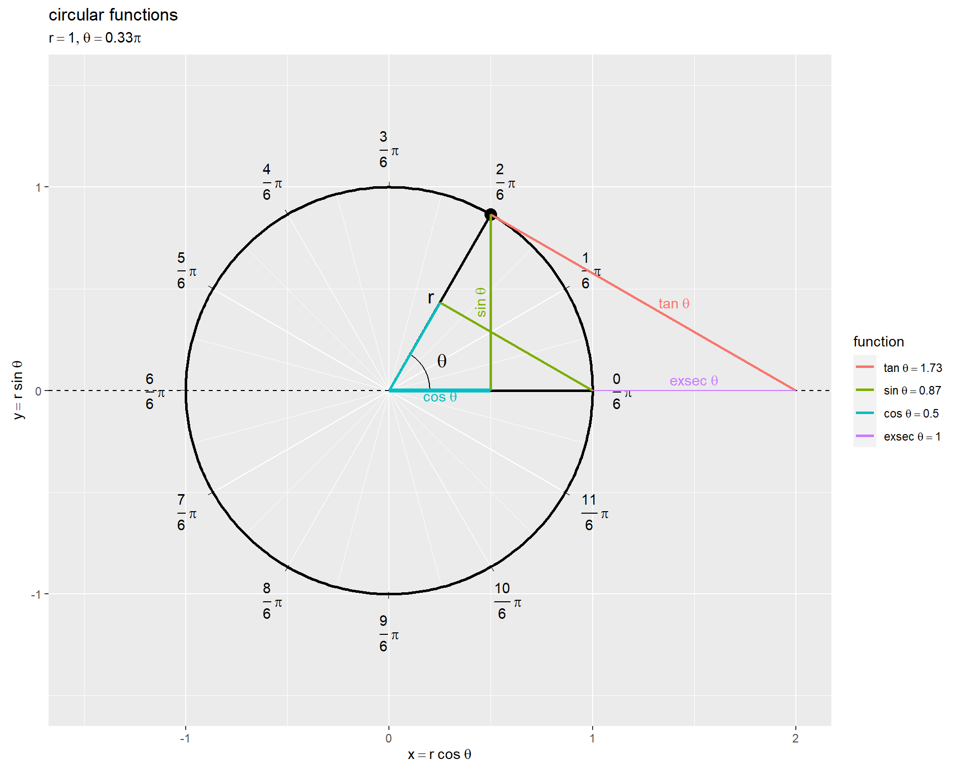
# ラベル用の文字列を作成
var_label <- paste0(
  "list(",
  "r == 1, ",
  "theta == ", round(theta/pi, digits = 2), " * pi",
  ")"
)
fnc_label_vec <- paste(
  c("tan~theta", "sin~theta", "cos~theta", "exsec~theta"),
  c(tan(theta), sin(theta), cos(theta), 1/cos(theta)-1) |>
    round(digits = 2),
  sep = " == "
)
var_label; fnc_label_vec
[1] "list(r == 1, theta == 0.33 * pi)"
[1] "tan~theta == 1.73" "sin~theta == 0.87" "cos~theta == 0.5"
[4] "exsec~theta == 1"
サブタイトル用の変数ラベル、凡例用の関数ラベルを作成します。
expression() の記法では、等号は "=="、複数の(数式上の)変数は "list(変数1, 変数2)" で並べて表示できます。
ここまでは、共通の処理です。ここからは、2つの方法で図示します。
パターン1
1つ目の方法では、x軸線から伸びる線分としてtan関数を可視化します。
・作図コード(クリックで展開)
関数を示す線分の描画用のデータフレームを作成します。
# 関数の描画順を指定
fnc_level_vec <- c("tan", "sin", "cos", "exsec")

# 関数線分の座標を作成
fnc_seg_df <- tibble::tibble(
  fnc = c("tan", "sin", "cos", "exsec") |>
    factor(levels = fnc_level_vec), # 関数カテゴリ
  x_from = c(
    1,
    cos(theta),
    0,
    cos(theta)
  ),
  y_from = c(
    0,
    0,
    0,
    sin(theta)
  ),
  x_to = c(
    1,
    cos(theta),
    cos(theta),
    1
  ),
  y_to = c(
    tan(theta),
    sin(theta),
    0,
    tan(theta)
  )
)
fnc_seg_df
# A tibble: 4 × 5
  fnc   x_from y_from  x_to  y_to
  <fct>  <dbl>  <dbl> <dbl> <dbl>
1 tan      1    0       1   1.73
2 sin      0.5  0       0.5 0.866
3 cos      0    0       0.5 0
4 exsec    0.5  0.866   1   1.73
各線分に対応する関数カテゴリを fnc 列として線の描き分けなどに使います。線分の描画順(重なり順)や色付け順を因子レベルで設定します。
各線分の始点の座標を x_from, y_from 列、終点の座標を x_to, y_to 列として、完成図を見ながら頑張って格納します。
関数ラベルの描画用のデータフレームを作成します。
# 関数ラベルの座標を作成
fnc_label_df <- tibble::tibble(
  fnc = c("tan", "sin", "cos", "exsec") |>
    factor(levels = fnc_level_vec), # 関数カテゴリ
  x = c(
    1,
    cos(theta),
    0.5 * cos(theta),
    0.5 * (cos(theta) + 1)
  ),
  y = c(
    0.5 * tan(theta),
    0.5 * sin(theta),
    0,
    0.5 * (sin(theta) + tan(theta))
  ),
  fnc_label = c("tan~theta", "sin~theta", "cos~theta", "exsec~theta"),
  a = c(90,  90,  0,   0),
  h = c(0.5, 0.5, 0.5, 1.1),
  v = c(1,  -0.5, 1,   0.5)
)
fnc_label_df
# A tibble: 4 × 7
  fnc       x     y fnc_label       a     h     v
  <fct> <dbl> <dbl> <chr>       <dbl> <dbl> <dbl>
1 tan    1    0.866 tan~theta      90   0.5   1
2 sin    0.5  0.433 sin~theta      90   0.5  -0.5
3 cos    0.25 0     cos~theta       0   0.5   1
4 exsec  0.75 1.30  exsec~theta     0   1.1   0.5
 関数ごとに1つの線分の中点に関数名を表示することにします。
関数ごとに1つの線分の中点に関数名を表示することにします。
ラベルの表示角度を a 列、表示角度に応じた左右の表示位置を h 列、上下の表示位置を v 列として指定します。
単位円におけるtan関数のグラフを作成します。
# グラフサイズの下限値・上限値を指定
axis_lower <- 1.5
axis_upper <- 3

# グラフサイズを設定
axis_x_size <- 1.5
axis_y_min  <- min(-axis_lower, tan(theta)) |> max(-axis_upper)
axis_y_max  <- max(axis_lower, tan(theta)) |> min(axis_upper)

# 単位円における関数線分を作図
ggplot() +
  geom_segment(data = rad_tick_df,
               mapping = aes(x = 0, y = 0, xend = x, yend = y, linewidth = grid),
               color = "white", show.legend = FALSE) + # 角度目盛線
  geom_text(data = rad_tick_df,
            mapping = aes(x = x, y = y, angle = a, label = tick_mark),
            size = 2) + # 角度目盛指示線
  geom_text(data = rad_tick_df,
            mapping = aes(x = label_x, y = label_y, label = rad_label, hjust = h, vjust = v),
            parse = TRUE) + # 角度目盛ラベル
  geom_path(data = circle_df,
            mapping = aes(x = x, y = y),
            linewidth = 1) + # 円周
  geom_segment(data = radius_df,
               mapping = aes(x = 0, y = 0, xend = x, yend = y),
               linewidth = 1) + # 半径線
  geom_path(data = angle_mark_df,
            mapping = aes(x = x, y = y)) + # 角マーク
  geom_text(data = angle_label_df,
            mapping = aes(x = x, y = y),
            label = "theta", parse = TRUE,
            size = 5) + # 角ラベル
  geom_text(mapping = aes(x = 0.5*cos(theta+0.1), y = 0.5*sin(theta+0.1)),
            label = "r", parse = TRUE,
            size = 5) + # 半径ラベル:(θ + αで表示位置を調整)
  geom_point(data = point_df,
             mapping = aes(x = x, y = y),
             size = 4) + # 円周上の点
  geom_vline(xintercept = 1, linetype = "dashed") + # 補助線
  geom_segment(data = fnc_seg_df,
               mapping = aes(x = x_from, y = y_from, xend = x_to, yend = y_to, color = fnc),
               linewidth = 1) + # 関数線分
  geom_text(data = fnc_label_df,
            mapping = aes(x = x, y = y, label = fnc_label, color = fnc,
                          hjust = h, vjust = v, angle = a),
            parse = TRUE, show.legend = FALSE) + # 関数ラベル
  scale_color_hue(labels = parse(text = fnc_label_vec), name = "function") + # 凡例表示用
  scale_linewidth_manual(breaks = c("major", "minor"),
                         values = c(0.5, 0.25)) + # 主・補助目盛線用
  theme(legend.text.align = 0) +
  coord_fixed(ratio = 1,
              xlim = c(-axis_x_size, axis_x_size),
              ylim = c(axis_y_min, axis_y_max)) +
  labs(title = "circular functions",
       subtitle = parse(text = var_label),
       x = expression(x == r ~ cos~theta),
       y = expression(y == r ~ sin~theta))
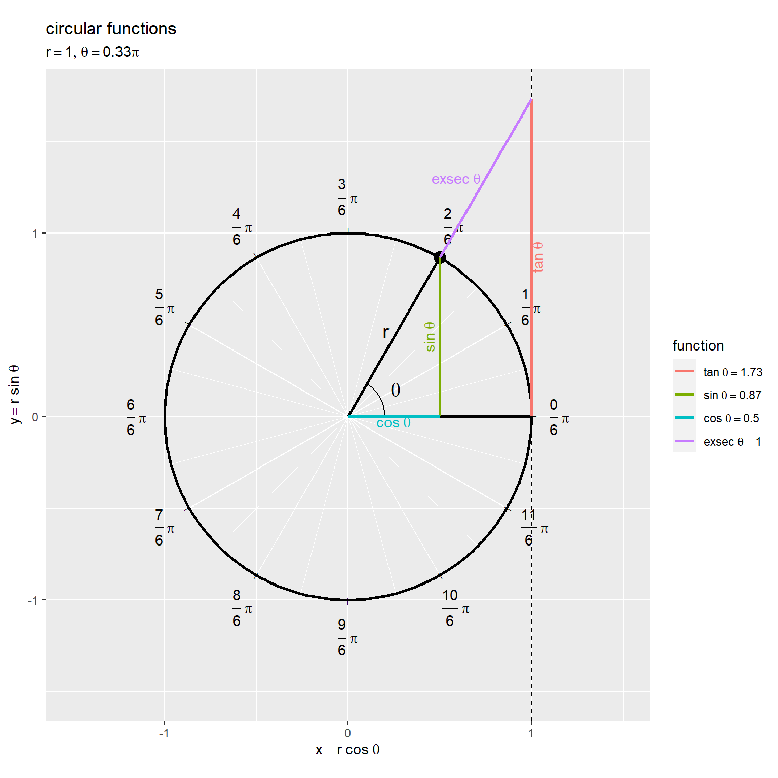
偏角(始線から動径までの反時計回りの角度)を として、単位円(
の円)の円周上の点の座標は
です。
tan関数の定義式 や、この図の相似な直角三角形の関係から、
なのが分かります。
に関する直角三角形について、隣辺(
に対応する辺)が1になるように拡大したときの対辺(
に対応する辺)と言えます。
よって、tan関数の値は、「原点と点 を通る半直線」と「
の直線」の交点のy座標(符号付きの高さ)です。
パターン2
2つ目の方法では、円周上の点から伸びる線分としてtan関数を可視化します。
・作図コード(クリックで展開)
関数を示す線分の描画用のデータフレームを作成します。
# 関数線分の座標を作成
fnc_seg_df <- tibble::tibble(
  fnc = c(
    "tan",
    "sin", "sin",
    "cos", "cos",
    "exsec"
  ) |>
    factor(levels = fnc_level_vec), # 関数カテゴリ
  x_from = c(
    cos(theta),
    cos(theta), abs(cos(theta))*cos(theta),
    0, 0,
    1
  ),
  y_from = c(
    sin(theta),
    0, abs(cos(theta))*sin(theta),
    0, 0,
    0
  ),
  x_to = c(
    1/cos(theta),
    cos(theta), ifelse(cos(theta) >= 0, yes = 1, no = -1),
    cos(theta), abs(cos(theta))*cos(theta),
    1/cos(theta)
  ),
  y_to = c(
    0,
    sin(theta), 0,
    0, abs(cos(theta))*sin(theta),
    0
  ),
  w = c(
    "normal",
    "normal", "normal",
    "bold", "normal",
    "thin"
  ) # 重なり対策用
)
fnc_seg_df
# A tibble: 6 × 6
  fnc   x_from y_from  x_to  y_to w
  <fct>  <dbl>  <dbl> <dbl> <dbl> <chr>
1 tan     0.5   0.866  2    0     normal
2 sin     0.5   0      0.5  0.866 normal
3 sin     0.25  0.433  1    0     normal
4 cos     0     0      0.5  0     bold
5 cos     0     0      0.25 0.433 normal
6 exsec   1     0      2    0     thin
「パターン1」と同様に、線分の座標を格納します。
関数ラベルの描画用のデータフレームを作成します。
# 関数ラベルの座標を作成
fnc_label_df <- tibble::tibble(
  fnc = c("tan", "sin", "cos", "exsec") |>
    factor(levels = fnc_level_vec), # 色用
  x = c(
    0.5 * (1/cos(theta) + cos(theta)),
    cos(theta),
    0.5 * cos(theta),
    0.5 * (1 + 1/cos(theta))
  ),
  y = c(
    0.5 * sin(theta),
    0.5 * sin(theta),
    0,
    0
  ),
  fnc_label = c("tan~theta", "sin~theta", "cos~theta", "exsec~theta"),
  a = c(0,    90,  0,   0),
  h = c(-0.5, 0.5, 0.5, 0.5),
  v = c(0.5, -0.5, 1,  -0.5)
)
fnc_label_df
# A tibble: 4 × 7
  fnc       x     y fnc_label       a     h     v
  <fct> <dbl> <dbl> <chr>       <dbl> <dbl> <dbl>
1 tan    1.25 0.433 tan~theta       0  -0.5   0.5
2 sin    0.5  0.433 sin~theta      90   0.5  -0.5
3 cos    0.25 0     cos~theta       0   0.5   1
4 exsec  1.5  0     exsec~theta     0   0.5  -0.5
線分の中点の座標とラベル用の文字列などを格納します。
単位円におけるtan関数のグラフを作成します。
# グラフサイズの下限値・上限値を指定
axis_lower <- 1.5
axis_upper <- 3

# グラフサイズを設定
axis_x_min  <- min(-axis_lower, 1/cos(theta)) |> max(-axis_upper)
axis_x_max  <- max(axis_lower, 1/cos(theta)) |> min(axis_upper)
axis_y_size <- 1.5

# 単位円における関数線分を作図
ggplot() +
  geom_segment(data = rad_tick_df,
               mapping = aes(x = 0, y = 0, xend = x, yend = y, linewidth = grid),
               color = "white", show.legend = FALSE) + # 角度目盛線
  geom_text(data = rad_tick_df,
            mapping = aes(x = x, y = y, angle = a, label = tick_mark),
            size = 2) + # 角度目盛指示線
  geom_text(data = rad_tick_df,
            mapping = aes(x = label_x, y = label_y, label = rad_label, hjust = h, vjust = v),
            parse = TRUE) + # 角度目盛ラベル
  geom_path(data = circle_df,
            mapping = aes(x = x, y = y),
            linewidth = 1) + # 円周
  geom_segment(data = radius_df,
               mapping = aes(x = 0, y = 0, xend = x, yend = y),
               linewidth = 1) + # 半径線
  geom_path(data = angle_mark_df,
            mapping = aes(x = x, y = y)) + # 角マーク
  geom_text(data = angle_label_df,
            mapping = aes(x = x, y = y),
            label = "theta", parse = TRUE,
            size = 5) + # 角ラベル
  geom_text(mapping = aes(x = 0.5*cos(theta+0.1), y = 0.5*sin(theta+0.1)),
            label = "r", parse = TRUE,
            size = 5) + # 半径ラベル:(θ + αで表示位置を調整)
  geom_point(data = point_df,
             mapping = aes(x = x, y = y),
             size = 4) + # 円周上の点
  geom_hline(yintercept = 0, linetype = "dashed") + # 補助線
  geom_segment(data = fnc_seg_df,
               mapping = aes(x = x_from, y = y_from, xend = x_to, yend = y_to,
                             color = fnc, linewidth = w)) + # 関数線分
  geom_text(data = fnc_label_df,
            mapping = aes(x = x, y = y, label = fnc_label, color = fnc,
                          hjust = h, vjust = v, angle = a),
            parse = TRUE, show.legend = FALSE) + # 関数ラベル
  scale_color_hue(labels = parse(text = fnc_label_vec), name = "function") + # 凡例表示用
  scale_linewidth_manual(breaks = c("bold", "normal", "thin", "major", "minor"),
                         values = c(1.5, 1, 0.5, 0.5, 0.25)) + # 重なり対策用, 主・補助目盛線用
  guides(color = guide_legend(override.aes = list(linewidth = 1)),
         linewidth = "none") +
  theme(legend.text.align = 0) +
  coord_fixed(ratio = 1,
              xlim = c(axis_x_min, axis_x_max),
              ylim = c(-axis_y_size, axis_y_size)) +
  labs(title = "circular functions",
       subtitle = parse(text = var_label),
       x = expression(x == r ~ cos~theta),
       y = expression(y == r ~ sin~theta))
動径(原点と円周上の点を結ぶ線分)を隣辺、x軸線の一部を斜辺としたときのパターン1の図と言えます。文字通り首を捻って見てください。
円周上の点を として、「動径に対する点
を通る垂線」と「
の直線」の交点を
とします。tan関数の値は、点
を結ぶ線分の符号付きの長さです。
アニメーションの作成
変数を変化させて、単位円におけるtan関数のアニメーションを作成します。
作図コードについては「tan_definition.R at anemptyarchive/Mathematics · GitHub」を参照してください。
・パターン1
(
は整数)(この図だと
の目盛位置)のとき
なので、動径が垂直になり直線
と平行(交点ができない)なため、
を描画(定義)できないのを確認できます。
・パターン2
こちらの図だと、動径の垂線が水平になり直線 と平行なため、
を描画(定義)できないのが分かります。
単位円と曲線の関係
最後は、単位円と関数曲線のグラフを作成して、変数(ラジアン)と座標の関係を可視化します。
作図コードについては「tan_definition.R」を参照してください。
変数と座標の関係
変数に応じて移動する円周上の点と曲線上の点のアニメーションを作成します。
点の座標
円周上の点とtan関数曲線上の点の関係を可視化します。
のとき曲線が不連続になり、その前後で符号(線分の向き)が変わるのを確認できます。
点の推移
円周上を周回した際のtan関数の推移を可視化します。
単位円を半周する の間隔で、曲線の形状が一致するのを確認できます。
この記事では、tan関数の定義を確認しました。次の記事からは、各種パラメータによる波形への影響を確認していきます。または、sec関数の定義を確認します。
参考書籍
- 『三角関数(改定第3版)』(Newton別冊)ニュートンプレス,2022年.
おわりに
cos関数で中断していた三角関数の可視化シリーズを、双曲線関数と線形代数(のベクトル編)を経由して、大幅バージョンアップして再開します。
相変わらず読ませる気が皆無な記事になりました。グラフとその解説だけを追うなり、コードをコピペするなりしてください。2つを繋げた図で、点やらが描画領域外に飛び出していますが仕様です。欠損値に置き換えるなどして対策できる(別記事ではした)のですが、これ以上コードがアレになってもアレなので、、
書いた本人的にはとても勉強になりました。 の周期は
だったんだな、解説書くまで気付かなかった。
そして!2023年5月7日は、元モーニング娘。の佐藤優樹さんの24歳のお誕生日です!
ソロデビュー共々おめでとうございます。
まーちゃんがいなければこのブログは存在しなかったと言っても過言ではないほどの存在です。ぜひこの曲を聴いてそれから他の曲も聴きましょう♪
ばぁ〜い
- 2024.03.21:加筆修正しました。
パラメータという呼び方をしていいのか分かりませんが振幅など曲線の変形の記事を書きたくて、その前に元の記事の構成などを整理しておこうというのが現在の修正作業の意図です。果たして力尽きずにそれぞれの関数で4記事(振幅・周期・位相の3つと全部)ずつ書けるのでしょうか。書けたらリンク張る用の枠がもう入ってます。
sin関数に関しては前回の更新時に基になる記事を書いていて(そこからかなり手を加えて再実装しましたが)、今回の修正を始める前にtan関数に関して実装しました。残り4関数×4パラ分、、、無理なのでは。
それに加えて(それらが面倒になって)、余角など角度系と、exsecやversinなどの派生関数系についてもいくつか作ってます。
つまりあれもこれも書きかけばかりが溜まっています。全部なんとかしたい。
【次の内容】