はじめに

　『スタンフォード　ベクトル・行列からはじめる最適化数学』の学習ノートです。
　「数式の行間埋め」や「Pythonを使っての再現」によって理解を目指します。本と一緒に読んでください。

　この記事は4.3節「k平均法」の内容です。
　多次元混合ガウス分布の乱数に対するk平均法によるクラスタリングを実装します。

【前の内容】

www.anarchive-beta.com

【他の内容】

www.anarchive-beta.com

【今回の内容】

はじめに
混合ガウス乱数のクラスタリング
- 2次元の場合
  - トイデータの作成
  - クラスタリング
- 3次元の場合
  - トイデータの生成
  - クラスタリング
参考書籍
おわりに

混合ガウス乱数のクラスタリング

　多次元混合ガウス分布(maltivariation gaussian mixture distribution)の乱数に対して、k平均法(k-means algorithm)によりクラスタリング(clustering)を行います。
　多次元混合ガウス分布については「多次元混合ガウス分布の定義式 - からっぽのしょこ」、代表値との距離については「【Python】3.2：最近傍の可視化【『スタンフォード線形代数入門』のノート】 - からっぽのしょこ」を参照してください。

　利用するライブラリを読み込みます。

# 利用ライブラリ
import numpy as np
from scipy.stats import multivariate_normal
import matplotlib.pyplot as plt
from matplotlib.animation import FuncAnimation

2次元の場合

　まずは、2次元空間(平面)上のベクトル(2次元のデータ)のクラスタリングを可視化します。

トイデータの作成

　クラスタリングを行う2次元混合ガウス分布の乱数を生成します。

・作図コード(クリックで展開)

　データの生成分布を設定します。

# 真のクラスタ数を指定
K_truth = 3

# K個の平均ベクトルを指定
mu = np.array(
    [[0.0, 5.0], 
     [5.0, -10.0], 
     [-10.0, -5.0]]
)

# K個の分散共分散行列を指定
sigma = np.array(
    [[[36.0, 10.0], [10.0, 25.0]], 
     [[9.0, -1.3], [-1.3, 16.0]], 
     [[25.0, -3.2], [-3.2, 16.0]]]
)

# 混合比率を指定
pi = np.array([0.45, 0.25, 0.3])

　真のクラスタ数 $K^{(\mathrm{truth})}$ を指定します。次元数(本では $n$ )は $D = 2$ とします。
　 $K^{(\mathrm{truth})}$ 個の平均ベクトル $\boldsymbol{\mu} = \{\boldsymbol{\mu}_1, \cdots, \boldsymbol{\mu}_{K^{(\mathrm{truth})}}\}$ と共分散行列 $\boldsymbol{\Sigma} = \{\boldsymbol{\Sigma}_1, \cdots, \boldsymbol{\Sigma}_{K^{(\mathrm{truth})}}\}$ をmu, sigmaとして値を指定します。クラスタ $j$ の平均ベクトルと分散共分散行列はそれぞれ次の形状です。

$\displaystyle \boldsymbol{\mu}_j = \begin{bmatrix} \mu_{j,1} \\ \mu_{j,2} \end{bmatrix} ,\ \boldsymbol{\Sigma}_j = \begin{bmatrix} \sigma_{j,2}^2 & \sigma_{j,1,2} \\ \sigma_{j,2,1} & \sigma_{j,2}^2 \end{bmatrix}$

　 $\mu_{j,d}$ は $c_i = j$ のときの(クラスタjのデータ) $x_{i,d}$ の平均、 $\sigma_{j,d} > 0$ は $x_{i,d}$ の標準偏差、 $\sigma_{j,d}^2 > 0$ は $x_{i,d}$ の分散、 $\sigma_{j,l,m} = \sigma_{j,m,l}$ は $x_{i,l}, x_{i,m}$ の共分散です。 $\boldsymbol{\Sigma}_j$ は正定値行列である必要があります。

　混合比率(クラスタの割り当て確率) $\boldsymbol{\pi} = (\pi_1, \cdots, \pi_{K^{(\mathrm{truth})}})^{\top}$ 、 $0 \leq \pi_j \leq 1$ 、 $\sum_{j=1}^K \pi_j = 1$ をpiとして値を指定します。

　確率密度の等高線を描画するのに使う点を作成します。データの生成自体には不要な処理です。

# 各軸の値を作成
x1_vals = np.linspace(
    np.min(mu[:, 0] - np.sqrt(sigma[:, 0, 0]) * 3.0), 
    np.max(mu[:, 0] + np.sqrt(sigma[:, 0, 0]) * 3.0), 
    num=300
)
x2_vals = np.linspace(
    np.min(mu[:, 1] - np.sqrt(sigma[:, 1, 1]) * 3.0), 
    np.max(mu[:, 1] + np.sqrt(sigma[:, 1, 1]) * 3.0), 
    num=300
)
print(x1_vals[:5].round(1))
print(x2_vals[:5].round(1))

# 作図用の点を作成
x1_grid, x2_grid = np.meshgrid(x1_vals, x2_vals)
print(x1_grid[:5, :5].round(1))
print(x2_grid[:5, :5].round(1))

# 作図用の点の形状を保存
x_dim = x1_grid.shape
print(x_dim)

# 計算用の点を作成
x_points = np.stack([x1_grid.flatten(), x2_grid.flatten()], axis=1)
print(x_points[:5].round(1))
print(x_points.shape)

[-25.  -24.9 -24.7 -24.6 -24.4]
[-22.  -21.9 -21.7 -21.6 -21.4]
[[-25.  -24.9 -24.7 -24.6 -24.4]
 [-25.  -24.9 -24.7 -24.6 -24.4]
 [-25.  -24.9 -24.7 -24.6 -24.4]
 [-25.  -24.9 -24.7 -24.6 -24.4]
 [-25.  -24.9 -24.7 -24.6 -24.4]]
[[-22.  -22.  -22.  -22.  -22. ]
 [-21.9 -21.9 -21.9 -21.9 -21.9]
 [-21.7 -21.7 -21.7 -21.7 -21.7]
 [-21.6 -21.6 -21.6 -21.6 -21.6]
 [-21.4 -21.4 -21.4 -21.4 -21.4]]
(300, 300)
[[-25.  -22. ]
 [-24.9 -22. ]
 [-24.7 -22. ]
 [-24.6 -22. ]
 [-24.4 -22. ]]
(90000, 2)

　この例では軸ごとに、平均を中心に標準偏差の3倍を範囲とします。
　軸ごとの値x*_valsを作成して、np.meshgrid()で格子状の点(全ての組み合わせ)x*_gridを作成します。また、x*_gridをそれぞれ列として結合して、2列の配列を作成します。
　x*_gridの同じインデックスの値、x_pointsの行が確率変数の値 $\mathbf{x} = (x_1, x_2)^{\top}$ に対応します。

　混合ガウス分布の確率密度を計算します。

# 確率密度を計算
dens = np.sum(
    [pi[j] * multivariate_normal.pdf(x=x_points, mean=mu[j], cov=sigma[j]) for j in range(K_truth)], 
    axis=0
)
print(dens[:5])
print(dens.shape)

[3.28052487e-10 3.63080417e-10 4.01620357e-10 4.43994078e-10
 4.90549144e-10]
(90000,)

　リスト内包表記のfor文を使って、クラスタごとに確率密度を計算し、混合比率を用いて加重平均を計算します。

$\displaystyle p(\mathbf{x}) = \sum_{j=1}^{K^{(\mathrm{truth})}} \pi_j \mathcal{N}(\mathbf{x} | \boldsymbol{\mu}_j, \boldsymbol{\Sigma}_j)$

　各クラスタの(混合ではない)多次元ガウス分布の確率密度は、SciPyライブラリのmultivariate_normalモジュールの確率密度関数pdf()で計算できます。確率変数の引数xに計算用の点x_points、平均ベクトルの引数meanに各クラスタの平均ベクトルmu[j]、分散共分散行列の引数covに各クラスタの分散共分散行列sugma[j]を指定します。

　各データに真のクラスタを割り当てます。

# データ数を指定
N = 100

# 真のクラスタを生成
c_truth_onehot = np.random.multinomial(n=1, pvals=pi, size=N)
print(c_truth_onehot[:5])
print(c_truth_onehot.shape)

# 真のクラスタ番号を抽出
_, c_truth = np.where(c_truth_onehot == 1)
print(c_truth[:5])
print(c_truth.shape)

# クラスタごとのデータ数を集計
G_num = np.sum(c_truth_onehot, axis=0)
print(G_num)
print(G_num.shape)

[[0 1 0]
 [0 0 1]
 [0 0 1]
 [1 0 0]
 [0 0 1]]
(100, 3)
[1 2 2 0 2]
(100,)
[47 23 30]
(3,)

　データ数(ベクトル数) $N$ を指定します。
　多項分布の乱数生成関数np.random.multinomial()の試行回数の引数nに1を指定して、カテゴリ分布の乱数を生成します。パラメータ(割り当て確率)の引数pvalsに混合比率pi、サンプルサイズの引数sizeにデータ数Nを指定します。
　one-hotベクトル(クラスタ番号に対応する列が1でそれ以外の列が0の行)をまとめたN行K_truth列の配列が出力されるので、np.where()で行ごとに値が1の列番号を抽出して、データごとの真のクラスタ番号 $\mathbf{c}^{(\mathrm{truth})} = (c_1^{(\mathrm{truth})}, \cdots, c_N^{(\mathrm{truth})})^{\top}$ 、 $c_i \in \{1, \dots, K^{(\mathrm{truth})}\}$ とします。
　各列の値が1の行数が、各クラスタが割り当てられたデータ数です。他の要素は0なので、列ごとの和で得られます。

　データ(ベクトル)を生成します。

# データを生成
X = np.array(
    [np.random.multivariate_normal(mean=mu[j], cov=sigma[j], size=1).flatten() for j in c_truth]
)
print(X[:5])
print(X.shape)

[[  4.76456936  -8.15120039]
 [-15.75284292  -3.86563593]
 [ -9.33917747  -6.14028522]
 [  7.06122445   6.89315561]
 [ -8.39557913 -10.8988496 ]]
(100, 2)

　クラス内包表記のfor文を使って、c_truthから順番にクラスタ番号を取り出して、対応するクラスタの多次元ガウス分布の乱数をnp.random.multivariate_normal()で生成します。平均ベクトルの引数meanに各クラスタの平均ベクトルmu[j]、分散共分散行列の引数covに各クラスタの分散共分散行列sigma[j]、サンプルサイズの引数sizeに1を指定します。
　N行2列の配列が出力されるので、データ $\mathbf{X} = \{\mathbf{x}_1, \cdots, \mathbf{x}_N\}$ 、 $\mathbf{x}_i = (x_{i,1}, x_{i,2})^{\top}$ とします。

　生成分布の等高線図とデータの散布図を作成します。

# 生成分布とデータを作図
fig, ax = plt.subplots(figsize=(12, 9), facecolor='white')
cnf = ax.contour(x1_grid, x2_grid, dens.reshape(x_dim), 
                 linestyles='--', zorder=0) # 生成分布
for j in range(K_truth):
    G_j, = np.where(c_truth == j) # クラスタjのデータインデック
    ax.scatter(x=X[G_j, 0], y=X[G_j, 1], s=50, label=str(j+1), zorder=1) # サンプルデータ
ax.set_title('N=' + str(N) + '=(' + ', '.join(map(str, G_num)) + ')', loc='left')
fig.suptitle('Gaussian mixture distribution', fontsize=20)
ax.set_xlabel('$x_1$')
ax.set_ylabel('$x_2$')
ax.grid()
ax.legend(title='cluster')
fig.colorbar(cnf, label='density')
ax.set_aspect('equal')
plt.show()

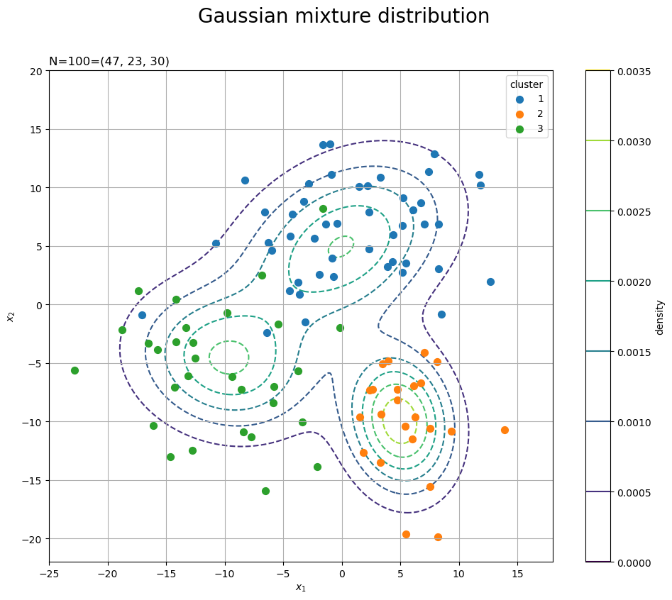
　混合多次元ガウス分布の確率密度の等高線をaxes.contour()で描画します。
　また、クラスタごとに多次元ガウス分布の乱数の散布図をaxes.scatter()で描画します。c_truthから値がjのインデックスを抽出してG_jとします。さらに、XからG_jに含まれる行を取り出して、色分けして描画します。

　目安として、目的関数を計算します。

# 目的関数(ノルムの2乗平均)を計算
J_truth = np.array(
    [np.sum(np.linalg.norm(X[c_truth == j] - mu[j], axis=1)**2) / N for j in range(K_truth)]
)
print(J_truth)

[27.01011683  5.88060014 17.64819944]

　生成分布の平均ベクトルを代表値として、「クラスタリング」で確認する目的関数 $J^{(\mathrm{clust})}$ と同様に、次の式を計算します。

$\displaystyle \begin{aligned} J^{(\mathrm{truth})} &= \sum_{j=1}^{K^{(\mathrm{truth})}} J_j^{(\mathrm{truth})} \\ J_j^{(\mathrm{truth})} &= \frac{1}{N} \sum_{i \in G_j^{(\mathrm{truth})}} \|\mathbf{x}_i - \boldsymbol{\mu}_{c_i^{(\mathrm{truth})}}\|^2 \end{aligned}$

　 $K^{(\mathrm{truth})}$ 個の $J_j^{(\mathrm{truth})}$ をJ_truthとしておき、作図時に $J^{(\mathrm{truth})}$ を計算します。 $G_j^{(\mathrm{truth})}$ は真のクラスタ $j$ の集合 $G_j^{(\mathrm{truth})} = \{j | c_i^{(\mathrm{truth})} = j\}$ を表します。
　 $\|\mathbf{x}\|$ は、ユークリッドノルムで、np.linalg.norm()で計算できます。

　真のクラスタをグラフで確認します。

# カラーマップを指定
cm = plt.get_cmap('gist_rainbow')
colors = cm(np.arange(K_truth) / K_truth)

# 2Dベクトルの真のクラスタを作図
fig, ax = plt.subplots(figsize=(12, 9), facecolor='white')
for j in range(K_truth):
    G_j, = np.where(c_truth == j) # クラスタjのデータのインデック
    ax.plot([mu[j, 0].repeat(len(G_j)), X[G_j, 0]], 
            [mu[j, 1].repeat(len(G_j)), X[G_j, 1]], 
            color=colors[j], linewidth=1, linestyle=':', zorder=0) # 対応線
    ax.scatter(x=mu[j, 0], y=mu[j, 1], 
               edgecolor=colors[j], facecolor='white', marker='s', s=100, zorder=1) # 平均値
    ax.scatter(x=X[G_j, 0], y=X[G_j, 1], 
               color=colors[j], s=20, label=str(j+1), zorder=2) # サンプルデータ
ax.set_title('N=' + str(N) + '=(' + ', '.join(map(str, G_num)) + '), ' + 
             'J=' + str(np.sum(J_truth).round(1)) + '=(' + ', '.join(map(str, J_truth.round(1))) + ')', loc='left')
fig.suptitle('true cluster', fontsize=20)
ax.set_xlabel('$x_1$')
ax.set_ylabel('$x_2$')
ax.grid()
ax.legend(title='cluster')
ax.set_aspect('equal')
plt.show()

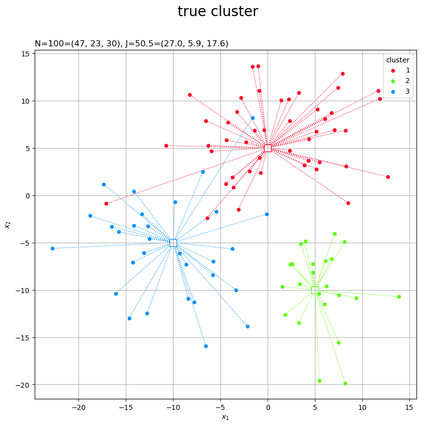
　各データを塗りつぶしの丸、真の平均値を白抜きの四角として描画します。
　クラスタごとに色分けするために、plt.get_cmap()にカラーマップ名を指定して、クラスタごとに色付けします。

　以上で、クラスタリングに利用する人工データを作成できました。

クラスタリング

　2次元ベクトルに対するk平均法を実装します。

　2通りの方法で初期値を設定できます。

　1つ目は、クラスタの初期値をランダムに割り当てて、クラスタごとに代表値として平均値を計算します。

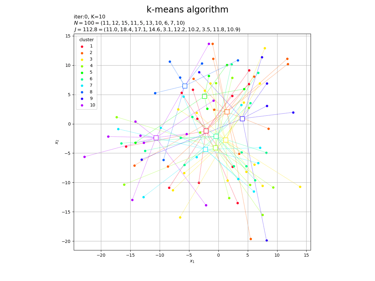
# クラスタ数の初期値を指定
K = 10

# ランダムにクラスタを割り当て
c_onehot = np.random.multinomial(n=1, pvals=np.repeat(1, K)/K, size=N)
print(c_onehot[:5])

# クラスタ番号を抽出
_, c = np.where(c_onehot == 1)
print(c[:5])

# クラスタごとのデータ数を集計
G_num = np.sum(c_onehot, axis=0)
print(G_num)

# クラスタの代表値(平均値)を計算
Z = np.array(
    [np.mean(X[c == j], axis=0) for j in range(K)]
)
print(Z[:5])

# 目的関数(ノルムの2乗平均)を計算
J = np.array(
    [np.sum(np.linalg.norm(X[c == j] - Z[j], axis=1)**2) / N for j in range(K)]
)
print(J[:5])

[[0 0 1 0 0 0 0 0 0 0]
 [1 0 0 0 0 0 0 0 0 0]
 [0 0 0 0 0 0 0 1 0 0]
 [0 0 1 0 0 0 0 0 0 0]
 [1 0 0 0 0 0 0 0 0 0]]
[2 0 7 2 0]
[11 12 15 11  5 13 10  6  7 10]
[[-2.11756701 -1.17656645]
 [ 1.45066723  2.03206318]
 [ 1.25141833 -2.75095687]
 [-0.49235447 -4.05065165]
 [-2.37184145  4.71364666]]
[10.97033869 18.36041448 17.14423579 14.55457911  3.09226981]

　本来は真のクラスタ数 $K^{(\mathrm{truth})}$ は分からないものなので、クラスタ数 $K$ の初期値を指定します。

　データの生成時と同様にして、データごとのクラスタ $\mathbf{c} = (c_1, \cdots, c_N)^{\top}$ 、 $c_i \in \{1, \dots, K\}$ の初期値を割り当てます。

　各クラスタが割り当てられたデータの平均値を代表値 $\mathbf{Z} = \{\mathbf{z}_1, \cdots, \mathbf{z}_K\}$ 、 $\mathbf{z}_j = (z_{j,1}, z_{j,2})^{\top}$ とします。

$\displaystyle z_{j,d} = \frac{1}{|G_j|} \sum_{i \in G_j} x_i$

　 $G_j$ は(初期値や推定値の)クラスタ $j$ の集合 $G_j = \{j | c_i = j\}$ 、 $|G_j|$ は $G_j$ の要素数を表します。
　各クラスタが割り当てられた要素数(データ数)は、データの生成時と同様にして、G_numとします。

　各データ $\mathbf{x}_i$ と割り当てられたクラスタの代表値 $\mathbf{z}_{c_i}$ の距離 $|\mathbf{x}_1 - \mathbf{z}_{c_1}|$ の2乗平均を目的関数とします。

$\displaystyle \begin{aligned} J^{(\mathrm{clust})} &= \frac{ \|\mathbf{x}_1 - \mathbf{z}_{c_1}\|^2 + \|\mathbf{x}_2 - \mathbf{z}_{c_2}\|^2 + \cdots + \|\mathbf{x}_N - \mathbf{z}_{c_N}\|^2 }{ N } \\ &= \sum_{j=1}^K J_j \\ J_j &= \frac{1}{N} \sum_{i \in G_j} \|\mathbf{x}_i - \mathbf{z}_{c_i}\|^2 \end{aligned}$

　 $K$ 個の $J_j$ をJとしておき、作図時に $J^{(\mathrm{clust})}$ を計算します。

　真のクラスタのときと同様にして、クラスタの初期値をグラフで確認します。

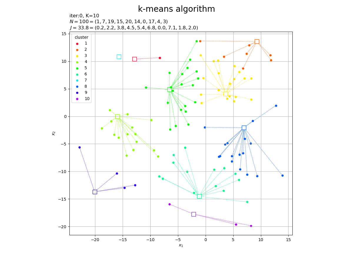
# カラーマップを指定
cm = plt.get_cmap('gist_rainbow')
colors = cm(np.arange(K) / K)

# 2Dベクトルのクラスタを作図
fig, ax = plt.subplots(figsize=(12, 9), facecolor='white')
for j in range(K):
    G_j, = np.where(c == j) # クラスタjのデータのインデック
    ax.plot([Z[j, 0].repeat(len(G_j)), X[G_j, 0]], 
            [Z[j, 1].repeat(len(G_j)), X[G_j, 1]], 
            color=colors[j], linewidth=1, linestyle=':', zorder=0) # 対応線
    ax.scatter(x=Z[j, 0], y=Z[j, 1], 
               edgecolor=colors[j], facecolor='white', marker='s', s=100) # 代表値
    ax.scatter(x=X[G_j, 0], y=X[G_j, 1], 
               color=colors[j], s=20, label=str(j+1)) # サンプルデータ
ax.set_title('iter:0, ' + 
             'N=' + str(N) + '=(' + ', '.join(str(val) for val in G_num) + '), ' + 
             'J=' + str(np.sum(J).round(1)) + '=(' + ', '.join(map(str, J.round(1))) + ')', loc='left')
fig.suptitle('initial cluster', fontsize=20)
ax.set_xlabel('$x_1$')
ax.set_ylabel('$x_2$')
ax.grid()
ax.legend(title='cluster')
ax.set_aspect('equal')
plt.show()

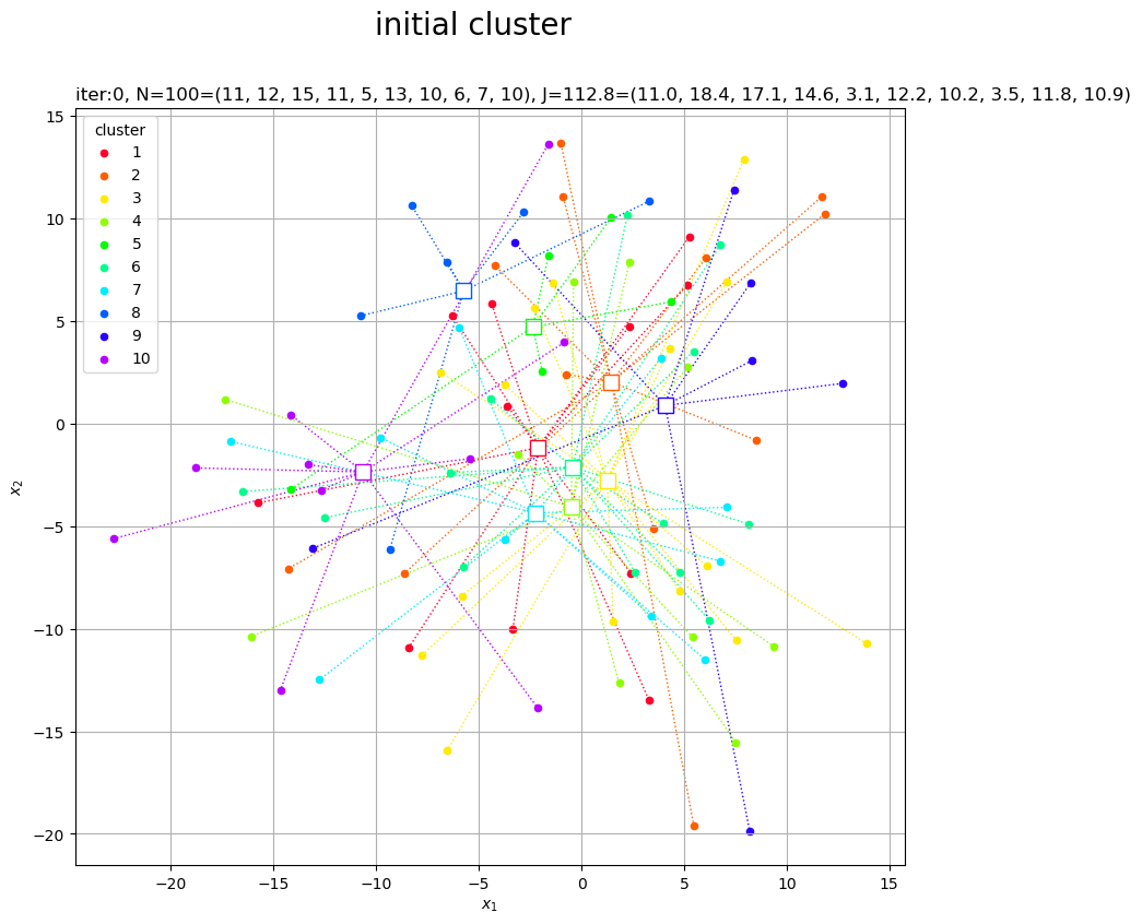
　ランダムに割り当てられたデータの平均値なので、代表値がデータ全体の中心付近に集まっています。

　2つ目は、代表値をランダムに設定して、データごとに代表値との距離が近い(ノルムが小さい)クラスタを割り当てます。

# クラスタ数の初期値を指定
K = 10

# ランダムにクラスタの代表値を設定
Z = np.array(
    [np.random.uniform(low=X[:, 0].min(), high=X[:, 0].max(), size=K), 
     np.random.uniform(low=X[:, 1].min(), high=X[:, 1].max(), size=K)]
).T
print(Z[:5])

# ノルムが最小のクラスタを割り当て
c = np.argmin(
    [np.linalg.norm(X - Z[j], axis=1) for j in range(K)], 
    axis=0
)
print(c[:5])

# クラスタごとのデータ数を集計
G_num = np.array(
    [np.sum(c == j) for j in range(K)]
)
print(G_num)

# 目的関数(ノルムの2乗平均)を計算
J = np.array(
    [np.sum(np.linalg.norm(X[c == j] - Z[j], axis=1)**2) / N for j in range(K)]
)
print(J[:5])

[[-12.86969694  10.39565196]
 [  9.29229126  13.58730506]
 [  3.62484662   4.05864789]
 [-15.96730452  -0.04264619]
 [ -6.55348377   4.85129958]]
[7 3 3 2 5]
[ 1  7 19 15 20 14  0 17  4  3]
[0.21124562 2.20122433 3.79361867 4.47382537 5.44145877]

　クラスタ数の初期値 $K$ を指定して、 $K$ 個の代表値 $\mathbf{z}_j$ の初期値をランダムに生成します。この例では、次元ごとに $\mathbf{x}_i$ の最小値から最大値を範囲として、np.random.uniform()で一様乱数を作成します。

　各データ $\mathbf{x}_i$ と各クラスタの代表値 $\mathbf{z}_j$ との距離 $\|\mathbf{x}_i - \mathbf{z}_j\|$ が最小となるクラスタ $j$ をそのデータのクラスタ $c_i$ とします。

$\displaystyle c_i = \mathop{\mathrm{argmin}}\limits_j \|\mathbf{x}_i - \mathbf{z}_j\| \quad (j = 1, 2, \dots, K)$

　最小値のインデックスはnp.argmin()で得られます。

　こちらの方法では、one-hotベクトルのクラスタ番号が不要なので、cに含まれる1からKの要素数をカウントして、クラスタごとのデータ数G_numとします。

　1つ目の方法と同じコードで、 $K$ 個の $J_j$ をJとして計算します。

　1つ目の方法と同じコードで、クラスタの初期値をグラフで確認します。

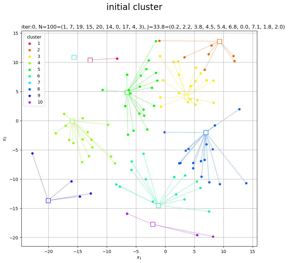
　代表値がばらけるので、ある程度まとまったクラスタができています。データが割り当てられないクラスタができることがあります。

　k平均法によりクラスタと代表値を繰り返し更新します。

# クラスタの最低割り当て数を指定
G_num_lower = 10

# 更新量の閾値を指定
threshold = 0.001

# 初期値を記録
trace_Z = [Z]
trace_c = [c]
trace_G = [G_num]
trace_J = [J]

# 繰り返し試行
cnt = 0
old_J_sum = np.sum(J)
while True:
    
    # 試行回数をカウント
    cnt += 1
    print('--- iter:' + str(cnt) + ' ---')
    
    # クラスタの代表値(平均値)を計算
    Z = np.array(
        [np.mean(X[c == j], axis=0) for j in range(K) if G_num[j] >= G_num_lower]
    )
    
    # クラスタ数を再設定
    K = len(Z)
    print('K=' + str(K))

    # ノルムが最小のクラスタを割り当て
    c = np.argmin(
        [np.linalg.norm(X - Z[j], axis=1) for j in range(K)], 
        axis=0
    )

    # クラスタごとのデータ数を集計
    G_num = np.array(
        [np.sum(c == j) for j in range(K)]
    )
    print('|G|=' + str(G_num))

    # 目的関数(ノルムの2乗平均)を計算
    J = np.array(
        [np.sum(np.linalg.norm(X[c == j] - Z[j], axis=1)**2) / N for j in range(K)]
    )
    J_sum = np.sum(J)
    print('J=' + str(J_sum.round(5)))
    
    # 更新値を記録
    trace_Z.append(Z)
    trace_c.append(c)
    trace_G.append(G_num)
    trace_J.append(J)
    
    # 更新量が閾値未満なら終了
    if abs(J_sum - old_J_sum) < threshold:
        break
    
    # 目的関数の値を保存
    old_J_sum = J_sum

--- iter:1 ---
K=5
|G|=[26 19 22 14 19]
J=28.81495
--- iter:2 ---
K=5
|G|=[25 19 24 13 19]
J=25.93017
--- iter:3 ---
K=5
|G|=[25 19 24 12 20]
J=25.6878
--- iter:4 ---
K=5
|G|=[25 19 24 10 22]
J=25.34453
--- iter:5 ---
K=5
|G|=[25 18 24  9 24]
J=24.64732
--- iter:6 ---
K=4
|G|=[25 23 25 27]
J=31.48424
--- iter:7 ---
K=4
|G|=[26 25 24 25]
J=30.02559
--- iter:8 ---
K=4
|G|=[26 26 23 25]
J=29.78286
--- iter:9 ---
K=4
|G|=[26 26 23 25]
J=29.74205
--- iter:10 ---
K=4
|G|=[26 26 23 25]
J=29.74205

　クラスタに含まれるデータ数が一定数未満になると、そのクラスタを削除することにします。
　下限値をG_num_lowerとして指定して、クラスタjのデータ数G_num[j]がG_num_lower以上のときのみ代表値(平均値)を計算します。クラスタが削除される(計算されないクラスタがある)と、クラスタ番号(行インデックス)が変わります。
　Zの行数をKとして、クラスタ数を更新します。

　クラスタの割り当てや、目的関数の計算については、これまでと同じです。

　閾値thresholdを指定し、前ステップの値をold_J_sumとしておき、更新値J_sumとの差の絶対値が閾値未満になると、収束したとみなしてbreakでループ処理を終了します。

　更新推移の確認用に、値(配列)をtrace_*に記録していきます。

　クラスタの更新値(収束結果)をグラフで確認します。

# カラーマップを指定
cm = plt.get_cmap('gist_rainbow')
colors = cm(np.arange(K) / K)

# 2Dベクトルのクラスタを作図
fig, ax = plt.subplots(figsize=(12, 9), facecolor='white')
for j in range(K):
    G_j, = np.where(c == j) # クラスタjのデータのインデック
    ax.plot([Z[j, 0].repeat(len(G_j)), X[G_j, 0]], 
            [Z[j, 1].repeat(len(G_j)), X[G_j, 1]], 
            color=colors[j], linewidth=1, linestyle=':', zorder=0) # 対応線
    ax.scatter(x=Z[j, 0], y=Z[j, 1], 
               edgecolor=colors[j], facecolor='white', marker='s', s=100) # 代表値
    ax.scatter(x=X[G_j, 0], y=X[G_j, 1], 
               color=colors[j], s=20, label=str(j+1)) # サンプルデータ
ax.set_title('iter:' + str(cnt) + ', ' + 
             'N=' + str(N) + '=(' + ', '.join(map(str, G_num)) + '), ' + 
             'J=' + str(np.sum(J).round(1)) + '=(' + ', '.join(map(str, J.round(1))) + ')', loc='left')
fig.suptitle('k-means algorithm', fontsize=20)
ax.set_xlabel('$x_1$')
ax.set_ylabel('$x_2$')
ax.grid()
ax.legend(title='cluster')
ax.set_aspect('equal')
plt.show()

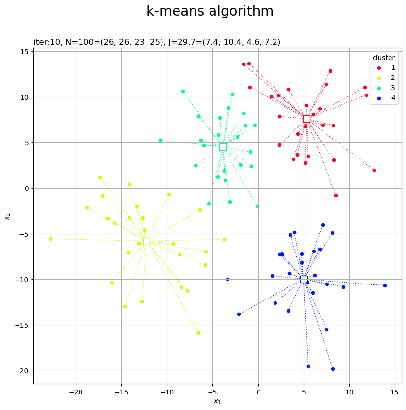
　これまでと同様にして作図します。

　目的関数の推移をグラフで確認します。

# 目的関数の推移を作図
fig, ax = plt.subplots(figsize=(8, 6), facecolor='white')
ax.plot(np.arange(cnt+1), [np.sum(J) for J in trace_J]) # 目的関数
ax.set_xlabel('iteration')
ax.set_ylabel('$J^{clust}$')
ax.set_title('N=' + str(N) + ', K=' + str(K), loc='left')
fig.suptitle('objective function', fontsize=20)
ax.grid()
plt.show()

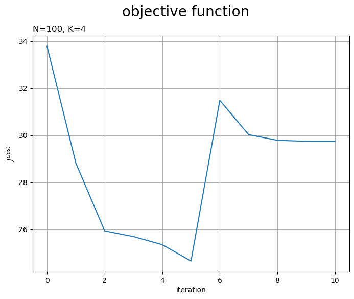
　試行の度に目的関数が下がるのを確認できます。ただし、クラスタ数の変更時には値が上がることがあります。

　更新の様子をアニメーションで確認します。

・作図コード(クリックで展開)

# フレーム数を設定
frame_num = cnt

# カラーマップを指定
cm = plt.get_cmap('gist_rainbow')
colors = cm(np.arange(len(trace_Z[0])) / len(trace_Z[0]))

# クラスタ数の削減に応じて色を入れ替え
colors_lt = [colors]
for i in range(frame_num):
    colors = colors[np.argsort(-np.int16(trace_G[i] >= G_num_lower))] # 継続するクラスタ番号の色を前に出す
    colors_lt.append(colors)

# グラフオブジェクトを初期化
fig, ax = plt.subplots(figsize=(12, 9), facecolor='white')
fig.suptitle('k-means algorithm', fontsize=20)

# 作図処理を関数として定義
def update(i):
    
    # 前フレームのグラフを初期化
    plt.cla()
    
    # i回目の値を取得
    Z = trace_Z[i]
    c = trace_c[i]
    G_num = trace_G[i]
    J = trace_J[i]
    colors = colors_lt[i]
    
    # クラスタ数を再設定
    K = len(Z)
    
    # 2Dベクトルのクラスタを作図
    for j in range(K):
        G_j, = np.where(c == j) # クラスタjのデータインデック
        ax.plot([Z[j, 0].repeat(len(G_j)), X[G_j, 0]], 
                [Z[j, 1].repeat(len(G_j)), X[G_j, 1]], 
                color=colors[j], linewidth=1, linestyle=':', zorder=0) # 対応線
        ax.scatter(x=Z[j, 0], y=Z[j, 1], 
                   edgecolor=colors[j], facecolor='white', marker='s', s=100) # 代表値
        ax.scatter(x=X[G_j, 0], y=X[G_j, 1], 
                   color=colors[j], s=20, label=str(j+1)) # サンプルデータ
    ax.set_title('iter:' + str(i) + ', ' + 
                 'K=' + str(K) + '\n' + 
                 '$N=' + str(N) + '=(' + ', '.join(map(str, G_num)) + ')$\n' + 
                 '$J=' + str(np.sum(J).round(1)) + '=(' + ', '.join(map(str, J.round(1))) + ')$', loc='left')
    ax.set_xlabel('$x_1$')
    ax.set_ylabel('$x_2$')
    ax.grid()
    ax.legend(title='cluster', loc='upper left')
    ax.set_aspect('equal')

# gif画像を作成
ani = FuncAnimation(fig=fig, func=update, frames=frame_num, interval=300)

# gif画像を保存
ani.save('k_means_gaussian_2d.gif')

　作図処理をupdate()として定義して、FuncAnimation()でgif画像を作成します。

3次元の場合

　次は、3次元空間上のベクトル(3次元のデータ)のクラスタリングを可視化します。

トイデータの生成

　クラスタリングを行う3次元混合ガウス分布の乱数を生成します。

・作図コード(クリックで展開)

　データの生成分布を設定します。

# 次元数を指定:(固定)
D = 3

# 真のクラスタ数を指定
K_truth = 3

# K個の平均ベクトルを指定
mu = np.array(
    [[0.0, -3.0, -3.0], 
     [3.0, 3.0, 0.0], 
     [-3.0, 3.0, 3.0]]
)

# K個の分散共分散行列を指定
sigma = np.array(
    [np.identity(D) * 3.0, 
     np.identity(D) * 3.0, 
     np.identity(D) * 3.0]
)

# 混合比率を指定
pi = np.array([0.45, 0.25, 0.3])

　次元数を $D = 3$ として、2次元のときと同様に、混合ガウス分布のパラメータと混合比率(クラスタの割り当て確率)を指定します。
　クラスタ $j$ の平均ベクトルと分散共分散行列はそれぞれ次の形状です。

$\displaystyle \boldsymbol{\mu}_j = \begin{bmatrix} \mu_{j,1} \\ \mu_{j,2} \\ \mu_{j,3} \end{bmatrix} ,\ \boldsymbol{\Sigma}_j = \begin{bmatrix} \sigma_{j,2}^2 & \sigma_{j,1,2} & \sigma_{j,1,3} \\ \sigma_{j,2,1} & \sigma_{j,2}^2 & \sigma_{j,2,3} \\ \sigma_{j,3,1} & \sigma_{j,3,2} & \sigma_{j,3}^2 \end{bmatrix}$

　各データに真のクラスタを割り当てます。

# データ数を指定
N = 100

# 真のクラスタを生成
c_truth_onehot = np.random.multinomial(n=1, pvals=pi, size=N)
print(c_truth_onehot[:5])

# 真のクラスタ番号を抽出
_, c_truth = np.where(c_truth_onehot == 1)
print(c_truth[:5])

# クラスタごとのデータ数を集計
G_num = np.sum(c_truth_onehot, axis=0)
print(G_num)

[[1 0 0]
 [0 1 0]
 [0 0 1]
 [0 0 1]
 [0 1 0]]
[0 1 2 2 1]
[42 24 34]

　「2次元の場合」と同じコードで、データごとに真のクラスタ $\mathbf{c}^{(\mathrm{truth})} = (c_1^{(\mathrm{truth})}, \cdots, c_N^{(\mathrm{truth})})^{\top}$ 、 $c_i \in \{1, \dots, K^{(\mathrm{truth})}\}$ を生成します。

　データ(ベクトル)を生成します。

# データを生成
X = np.array([
    np.random.multivariate_normal(mean=mu[j], cov=sigma[j], size=1).flatten() for j in c_truth
])
print(X[:5])

[[-0.9061569  -3.07634996 -2.36736738]
 [ 3.83759876  3.80356171  2.01786429]
 [-0.0631905   2.22261667  1.1232106 ]
 [-0.01111482  4.86771311  0.96188149]
 [ 7.40436435  1.09319964  0.55241717]]

　「2次元の場合」と同じコードで、割り当てられたクラスタに応じてデータ $\mathbf{X} = \{\mathbf{x}_1, \cdots, \mathbf{x}_N\}$ 、 $\mathbf{x}_i = (x_{i,1}, x_{i,2}, x_{i,3})^{\top}$ を生成します。

　データと真のクラスタを散布図で確認します。

# 目的関数(ノルムの2乗平均)を計算
J_truth = np.array(
    [np.sum(np.linalg.norm(X[c_truth == j] - mu[j], axis=1)**2) / N for j in range(K_truth)]
)

# カラーマップを指定
cm = plt.get_cmap('gist_rainbow')
colors = cm(np.arange(K_truth) / K_truth)

# サイズ用の値を設定
z_min = X[:, 2].min() + 1
z_max = X[:, 2].max() + 1

# 3Dベクトルの真のクラスタを作図
fig, ax = plt.subplots(figsize=(12, 9), facecolor='white', 
                       subplot_kw={'projection': '3d'})
for j in range(K_truth):
    G_j, = np.where(c_truth == j) # クラスタjのデータインデック
    ax.quiver(*np.tile(mu[j], reps=(len(G_j), 1)).T, 
              *(X[G_j]-mu[j]).T, color=colors[j], 
              arrow_length_ratio=0.0, linewidth=0.5, linestyle=':') # 対応線
    ax.scatter(*mu[j].T, 
               edgecolor=colors[j], facecolor='white', marker='s', s=100, zorder=1) # 平均値
    ax.scatter(*X[G_j].T, 
               color=colors[j], s=20, label=str(j+1), zorder=2) # サンプルデータ
ax.quiver(mu[:, 0], mu[:, 1], mu[:, 2], 
          np.zeros(K_truth), np.zeros(K_truth), z_min-mu[:, 2], 
          color='gray', arrow_length_ratio=0, linestyle=':') # 補助線
ax.set_title('N=' + str(N) + '=(' + ', '.join(map(str, G_num)) + '), ' + 
             'J=' + str(np.sum(J_truth).round(1)) + '=(' + ', '.join(map(str, J_truth.round(1))) + ')', loc='left')
fig.suptitle('true cluster', fontsize=20)
ax.set_xlabel('$x_1$')
ax.set_ylabel('$x_2$')
ax.set_zlabel('$x_3$')
ax.legend(title='cluster')
ax.set_zlim(z_min, z_max)
plt.show()

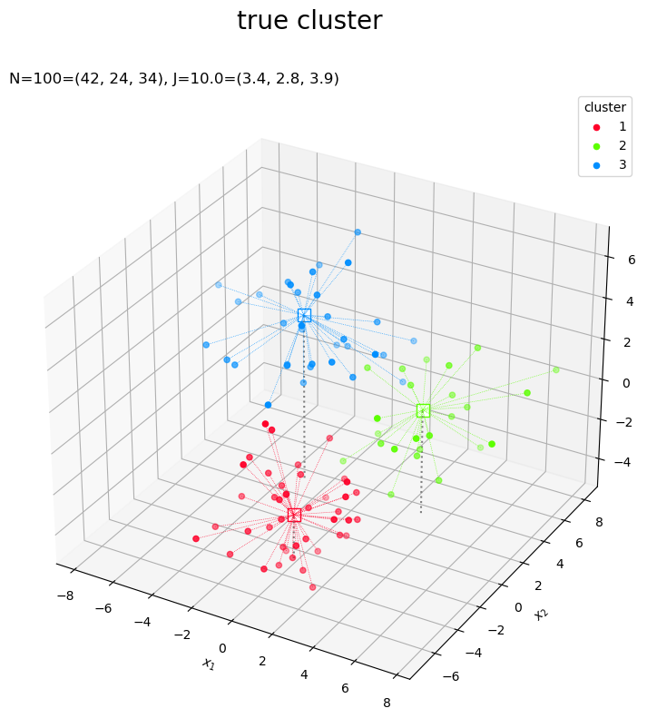
　各データを塗りつぶしの丸、真の平均値を白抜きの四角として描画します。
　クラスタごとの代表値と各データを結ぶ線分を(3Dプロットだとaxes.plot()でまとめて描画できなかった？ので)axes.quiver()で描画します。第1・2・3引数に始点の座標、第4・5・6引数に変化量(ベクトルのサイズ)を指定します。
　それぞれ、配列の前に*を付けてアンパック(展開)して指定しています。

　以上で、クラスタリングに利用する人工データを作成できました。

クラスタリング

　3次元ベクトルに対するk平均法を実装します。

　2通りの方法で初期値を設定できます。

　1つ目は、クラスタの初期値をランダムに割り当てて、クラスタごとに代表値として平均値を計算します。

# クラスタ数の初期値を指定
K = 10

# ランダムにクラスタを割り当て
c_onehot = np.random.multinomial(n=1, pvals=np.repeat(1, K)/K, size=N)
print(c_truth_onehot[:5])

# クラスタ番号を抽出
_, c = np.where(c_onehot == 1)
print(c[:5])

# クラスタごとのデータ数を集計
G_num = np.sum(c_onehot, axis=0)
print(G_num)

# クラスタの代表値(平均値)を計算
Z = np.array(
    [np.mean(X[c == j], axis=0) for j in range(K)]
)
print(Z[:5])

# 目的関数(ノルムの2乗平均)を計算
J = np.array(
    [np.sum(np.linalg.norm(X[c == j] - Z[j], axis=1)**2) / N for j in range(K)]
)
print(J[:5])

[[0 0 0 0 1 0 0 0 0 0]
 [0 0 0 0 1 0 0 0 0 0]
 [0 0 0 0 0 0 0 0 1 0]
 [0 0 0 0 0 0 0 1 0 0]
 [0 0 1 0 0 0 0 0 0 0]]
[5 5 8 7 2]
[ 8  2 10 10  9 17 10 16  7 11]
[[-0.83196199 -0.71145777 -0.20413865]
 [-1.80777768 -2.11801431 -0.68183497]
 [ 0.98736262  1.46167339  0.72020464]
 [ 0.06203712 -0.47859545 -1.06351002]
 [-1.0299771   0.71466154  0.25949943]]
[1.55461591 0.29448437 2.69100556 2.68898349 1.96192039]

　「2次元の場合」と同じコードで、クラスタ $\mathbf{c} = (c_1, \cdots, c_N)^{\top}$ 、 $c_i \in \{1, \dots, K\}$ と代表値 $\mathbf{Z} = \{\mathbf{z}_1, \cdots, \mathbf{z}_K\}$ 、 $\mathbf{z}_j = (z_{j,1}, z_{j,2}, z_{j,3})^{\top}$ を初期化します。

　真のクラスタのときと同様にして、クラスタの初期値をグラフで確認します。

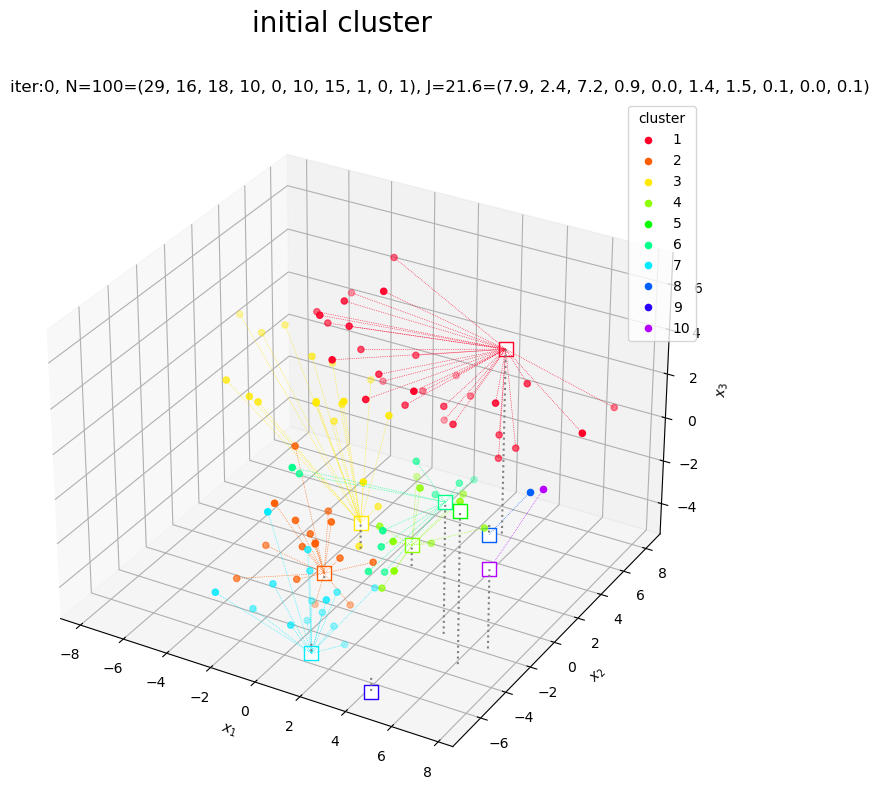
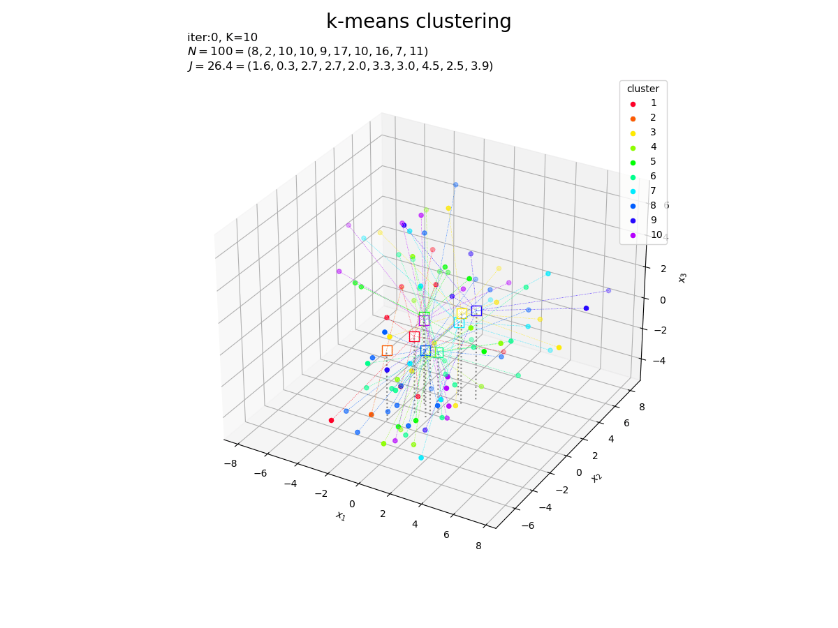
# カラーマップを指定
cm = plt.get_cmap('gist_rainbow')
colors = cm(np.arange(K) / K)

# サイズ用の値を設定
z_min = X[:, 2].min() + 1
z_max = X[:, 2].max() + 1

# 3Dベクトルのクラスタを作図
fig, ax = plt.subplots(figsize=(12, 9), facecolor='white', 
                       subplot_kw={'projection': '3d'})
for j in range(K):
    G_j, = np.where(c == j) # クラスタjのデータインデック
    ax.quiver(*np.tile(Z[j], reps=(len(G_j), 1)).T, 
              *(X[G_j]-Z[j]).T, color=colors[j], 
              arrow_length_ratio=0.0, linewidth=0.5, linestyle=':') # 対応線
    ax.scatter(*Z[j].T, 
               edgecolor=colors[j], facecolor='white', marker='s', s=100, zorder=1) # 平均値
    ax.scatter(*X[G_j].T, 
               color=colors[j], s=20, label=str(j+1), zorder=2) # サンプルデータ
ax.quiver(Z[:, 0], Z[:, 1], Z[:, 2], 
          np.zeros(K), np.zeros(K), z_min-Z[:, 2], 
          color='gray', arrow_length_ratio=0, linestyle=':') # 補助線
ax.set_title('iter:0, ' + 
             'N=' + str(N) + '=(' + ', '.join(map(str, G_num)) + '), ' + 
             'J=' + str(np.sum(J).round(1)) + '=(' + ', '.join(map(str, J.round(1))) + ')', loc='left')
fig.suptitle('initial cluster', fontsize=20)
ax.set_xlabel('$x_1$')
ax.set_ylabel('$x_2$')
ax.set_zlabel('$x_3$')
ax.legend(title='cluster')
ax.set_zlim(z_min, z_max)
ax.set_aspect('equal')
plt.show()

　ランダムに割り当てられたデータの平均値なので、代表値がデータ全体の中心付近に集まっています。

　2つ目は、代表値をランダムに設定して、データごとに代表値との距離が近い(ノルムが小さい)クラスタを割り当てます。

# クラスタ数の初期値を指定
K = 10

# ランダムにクラスタの代表値を設定
Z = np.array(
    [np.random.uniform(low=X[:, 0].min(), high=X[:, 0].max(), size=K), 
     np.random.uniform(low=X[:, 1].min(), high=X[:, 1].max(), size=K), 
     np.random.uniform(low=X[:, 2].min(), high=X[:, 2].max(), size=K)]
).T
print(Z[:5])

# ノルムが最小のクラスタを割り当て
c = np.argmin(
    [np.linalg.norm(X - Z[j], axis=1) for j in range(K)], 
    axis=0
)
print(c[:5])

# クラスタごとのデータ数を集計
G_num = np.array(
    [np.sum(c == j) for j in range(K)]
)
print(G_num)

# 目的関数(ノルムの2乗平均)を計算
J = np.array(
    [np.sum(np.linalg.norm(X[c == j] - Z[j], axis=1)**2) / N for j in range(K)]
)
print(J[:5])

[[ 3.22789816  5.73999796  3.33690734]
 [-1.28032404 -0.79235536 -4.94935583]
 [-1.14602146  1.86271125 -3.97244374]
 [ 1.28276238  1.73445996 -4.20285614]
 [ 6.29835174 -3.55930852  1.68244032]]
[1 0 2 0 9]
[29 16 18 10  0 10 15  1  0  1]
[7.89345639 2.37520645 7.21887148 0.94524146 0.        ]

　代表値Zとして、K行3列の一様乱数を生成します。
　それ以外は「2次元の場合」と同じコードで初期化できます。

　1つ目の方法と同じコードで、クラスタの初期値をグラフで確認します。

　代表値がばらけるので、ある程度まとまったクラスタができています。データが割り当てられないクラスタができることがあります。

　k平均法によりクラスタと代表値を繰り返し更新します。

--- iter:1 ---
K=6
|G|=[24 13 20 16 10 17]
J=8.92923
--- iter:2 ---
K=6
|G|=[21 17 22 16  8 16]
J=7.70315
--- iter:3 ---
K=5
|G|=[17 19 27 19 18]
J=8.02358
--- iter:4 ---
K=5
|G|=[18 19 27 17 19]
J=7.39068
--- iter:5 ---
K=5
|G|=[18 19 27 17 19]
J=7.35017
--- iter:6 ---
K=5
|G|=[18 19 27 17 19]
J=7.35017

　「2次元の場合」のコードで処理できます。

　クラスタの更新値(収束結果)をグラフで確認します。

# カラーマップを指定
cm = plt.get_cmap('gist_rainbow')
colors = cm(np.arange(K) / K)

# サイズ用の値を設定
z_min = X[:, 2].min() + 1
z_max = X[:, 2].max() + 1

# 3Dベクトルのクラスタを作図
fig, ax = plt.subplots(figsize=(12, 9), facecolor='white', 
                       subplot_kw={'projection': '3d'})
for j in range(K):
    G_j, = np.where(c == j) # クラスタkのデータインデック
    ax.quiver(*np.tile(Z[j], reps=(len(G_j), 1)).T, 
              *(X[G_j]-Z[j]).T, color=colors[j], 
              arrow_length_ratio=0.0, linewidth=0.5, linestyle=':') # 対応線
    ax.scatter(*Z[j].T, 
               edgecolor=colors[j], facecolor='white', marker='s', s=100, zorder=1) # 代表値
    ax.scatter(*X[G_j].T, 
               color=colors[j], s=20, label=str(j+1), zorder=2) # サンプルデータ
ax.quiver(Z[:, 0], Z[:, 1], Z[:, 2], 
          np.zeros(K), np.zeros(K), z_min-Z[:, 2], 
          color='gray', arrow_length_ratio=0, linestyle=':') # 補助線
ax.set_title('iter:' + str(cnt) + ', ' + 
             'N=' + str(N) + '=(' + ', '.join(map(str, G_num)) + '), ' + 
             'J=' + str(np.sum(J_truth).round(1)) + '=(' + ', '.join(map(str, J_truth.round(1))) + ')', loc='left')
fig.suptitle('k-means clustering', fontsize=20)
ax.set_xlabel('$x_1$')
ax.set_ylabel('$x_2$')
ax.set_zlabel('$x_3$')
ax.legend(title='cluster')
ax.set_zlim(z_min, z_max)
ax.set_aspect('equal')
plt.show()

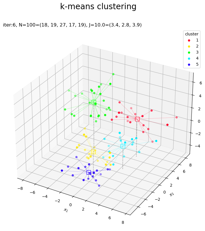
　これまでと同様にして作図します。

　目的関数の推移をグラフで確認します。

# 目的関数の推移を作図
fig, ax = plt.subplots(figsize=(8, 6), facecolor='white')
ax.plot(np.arange(cnt+1), [np.sum(J) for J in trace_J]) # 目的関数
ax.grid()
ax.set_xlabel('iteration')
ax.set_ylabel('$J^{clust}$')
ax.set_title('N=' + str(N) + ', K=' + str(K), loc='left')
fig.suptitle('objective function', fontsize=20)
plt.show()

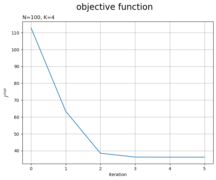
　試行の度に目的関数が下がるのを確認できます。ただし、クラスタ数の変更時には値が上がることがあります。

　更新の様子をアニメーションで確認します。

・作図コード(クリックで展開)

# フレーム数を設定
frame_num = cnt

# カラーマップを指定
cm = plt.get_cmap('gist_rainbow')
colors = cm(np.arange(len(trace_Z[0])) / len(trace_Z[0]))

# クラスタ数の削減に応じて色を入れ替え
colors_lt = [colors]
for i in range(frame_num):
    colors = colors[np.argsort(-np.int16(trace_G[i] >= G_num_lower))] # 継続するクラスタ番号の色を前に出す
    colors_lt.append(colors)

# サイズ用の値を設定
z_min = X[:, 2].min() + 1
z_max = X[:, 2].max() + 1

# グラフオブジェクトを初期化
fig, ax = plt.subplots(figsize=(12, 9), facecolor='white', 
                       subplot_kw={'projection': '3d'})
fig.suptitle('k-means clustering', fontsize=20)

# 作図処理を関数として定義
def update(i):
    
    # 前フレームのグラフを初期化
    plt.cla()
    
    # i回目の値を取得
    Z = trace_Z[i]
    c = trace_c[i]
    G_num = trace_G[i]
    J = trace_J[i]
    colors = colors_lt[i]
    
    # クラスタ数を再設定
    K = len(Z)
    
    # 3Dベクトルのクラスタを作図
    for j in range(K):
        G_j, = np.where(c == j) # クラスタjのデータインデック
        ax.quiver(*np.tile(Z[j], reps=(len(G_j), 1)).T, 
                  *(X[G_j]-Z[j]).T, color=colors[j], 
                  arrow_length_ratio=0.0, linewidth=0.5, linestyle=':') # 対応線
        ax.scatter(*Z[j].T, 
                   edgecolor=colors[j], facecolor='white', marker='s', s=100, zorder=1) # 代表値
        ax.scatter(*X[G_j].T, 
                   color=colors[j], s=20, label=str(j+1), zorder=2) # サンプルデータ
    ax.quiver(Z[:, 0], Z[:, 1], Z[:, 2], 
              np.zeros(K), np.zeros(K), z_min-Z[:, 2], 
              color='gray', arrow_length_ratio=0, linestyle=':') # 補助線
    ax.set_title('iter:' + str(i) + ', ' + 
                 'K=' + str(K) + '\n' + 
                 '$N=' + str(N) + '=(' + ', '.join(map(str, G_num)) + ')$\n' + 
                 '$J=' + str(np.sum(J).round(1)) + '=(' + ', '.join(map(str, J.round(1))) + ')$', loc='left')
    ax.set_xlabel('$x_1$')
    ax.set_ylabel('$x_2$')
    ax.set_zlabel('$x_3$')
    ax.legend(title='cluster')
    ax.set_zlim(z_min, z_max)

# gif画像を作成
ani = FuncAnimation(fig=fig, func=update, frames=frame_num, interval=300)

# gif画像を保存
ani.save('k_means_gaussian_3d.gif')