はじめに

　『スタンフォード　ベクトル・行列からはじめる最適化数学』の学習ノートです。
　「数式の行間埋め」や「Pythonを使っての再現」によって理解を目指します。本と一緒に読んでください。

　この記事は1.3節「ベクトルスカラー積」の内容です。
　標準単位ベクトルの線形結合を可視化します。

【前の内容】

www.anarchive-beta.com

【他の内容】

www.anarchive-beta.com

【今回の内容】

はじめに
標準単位ベクトルの線形結合の可視化
- 2次元の場合
- 3次元の場合
参考書籍
おわりに

標準単位ベクトルの線形結合の可視化

　標準単位ベクトル(canonical unit vector)を用いた線形結合(linear combination)をグラフで確認します。
　線形結合については「【Python】1.3：ベクトルの線形結合の例【『スタンフォード線形代数入門』のノート】 - からっぽのしょこ」を参照してください。

　利用するライブラリを読み込みます。

# 利用ライブラリ
import numpy as np
import matplotlib.pyplot as plt
from matplotlib.animation import FuncAnimation

2次元の場合

　まずは、2次元空間(平面)上でベクトルの線形結合を可視化します。

　2次元ベクトルと標準単位ベクトルを指定します。

# ベクトルを指定
a = np.array([4.5, 3.6])

# 係数を指定
e1 = np.array([1.0, 0.0])
e2 = np.array([0.0, 1.0])

　 $\mathbf{a} = (a_1, a_2)^{\top}$ をa、 $\mathbf{e}_1 = (1, 0)^{\top}, \mathbf{e}_2 = (0, 1)^{\top}$ をe1, e2として値を指定します。ただし、Pythonでは0からインデックスが割り当てられるので、 $a_1$ の値はa[0]に対応します。

　2次元空間上に3つのベクトル $\mathbf{a}, \mathbf{e}_1, \mathbf{e}_2$ を描画します。

# 作図用の値を設定
x_min = np.floor(np.min([0.0, a[0]])) - 1
x_max = np.ceil(np.max([1.0, a[0]])) + 1
y_min = np.floor(np.min([0.0, a[1]])) - 1
y_max = np.ceil(np.max([1.0, a[1]])) + 1

# (原点からの)2Dベクトルを作図
fig, ax = plt.subplots(figsize=(6, 4.5), facecolor='white')
ax.quiver(0, 0, *a, angles='xy', scale_units='xy', scale=1) # ベクトルa
ax.quiver(0, 0, *e1, color='red', angles='xy', scale_units='xy', scale=1) # ベクトルe1
ax.quiver(0, 0, *e2, color='blue', angles='xy', scale_units='xy', scale=1) # ベクトルe2
ax.annotate(xy=0.5*a, text='a', size=15, ha='right', va='bottom') # ベクトルaラベル
ax.annotate(xy=0.5*e1, text='$e_1$', size=10, ha='center', va='top') # ベクトルe1ラベル
ax.annotate(xy=0.5*e2, text='$e_2$', size=10, ha='right', va='center') # ベクトルe2ラベル
ax.set_xticks(ticks=np.arange(x_min, x_max+1))
ax.set_yticks(ticks=np.arange(y_min, y_max+1))
ax.grid()
ax.set_xlabel('x')
ax.set_ylabel('y')
ax.set_title('a=('+', '.join(map(str, a))+')', loc='left')
fig.suptitle('$a, e_1, e_2$', fontsize=20)
ax.set_aspect('equal')
plt.show()

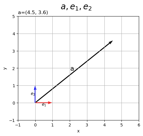
　各ベクトルのグラフをaxes.quiver()で描画します。第1・2引数に始点の座標、第3・4引数にベクトルのサイズ(変化量)を指定します。この例では、原点を始点とします。
　配列a, e1, e2の前に*を付けてアンパック(展開)して指定しています。

　 $a_1 \mathbf{e}_1 + a_2 \mathbf{e}_2$ のベクトルを描画します。

# 符号を取得
sign_x = np.sign(a[0])
sign_y = np.sign(a[1])

# 単位ベクトルの数を設定
num_x = int(np.ceil(abs(a[0])))
num_y = int(np.ceil(abs(a[1])))

# ラベル用のリストを作成
sign_str_lt = ['', '0', '-']

# 2D標準単位ベクトルの線形結合を作図
fig, ax = plt.subplots(figsize=(6, 5), facecolor='white')
ax.quiver(0, 0, *a, angles='xy', scale_units='xy', scale=1) # ベクトルa
for j in range(num_x):
    if j+1 <= abs(a[0]):
        # x軸方向の単位ベクトルを描画
        ax.quiver(sign_x*j, 0, *sign_x*e1, color='red', 
                  angles='xy', scale_units='xy', scale=1) # ベクトルe1
    else:
        # x軸方向の差分のベクトルを描画
        diff_x = a[0] - sign_x * j
        ax.quiver(sign_x*j, 0, diff_x, e1[1], color='red', 
                  angles='xy', scale_units='xy', scale=1) # ベクトルw1e1
        ax.annotate(xy=[sign_x*j+0.5*diff_x, e1[1]], text='$'+str(diff_x.round(2))+'e_1$', 
                    size=10, ha='center', va='top') # ベクトルw2e1ラベル
for k in range(num_y):
    if k+1 <= abs(a[1]):
        # y軸方向の単位ベクトルを描画
        ax.quiver(a[0], sign_y*k, *sign_y*e2, color='blue', 
                  angles='xy', scale_units='xy', scale=1) # ベクトルe2
    else:
        # y軸方向の差分のベクトルを描画
        diff_y = a[1] - sign_y * k
        ax.quiver(a[0], sign_y*k, e2[0], diff_y, color='blue', 
                  angles='xy', scale_units='xy', scale=1) # ベクトルw2e2
        ax.annotate(xy=[a[0], sign_y*k+0.5*diff_y], text='$'+str(diff_y.round(2))+'e_2$', 
                    size=10, ha='left', va='center') # ベクトルw2e2ラベル
ax.annotate(xy=0.5*a, text='a', 
            size=15, ha='right', va='bottom') # ベクトルaラベル
if abs(a[0]) >= 1.0 or a[0] == 0.0:
    sign_x_str = [sign_str_lt[idx] for idx, bl in enumerate([a[0] >= 1.0, a[0] == 0.0, a[0] <= -1.0]) if bl][0]
    ax.annotate(xy=sign_x*0.5*e1, text='$'+sign_x_str+'e_1$', 
                size=10, ha='center', va='top') # ベクトルe1ラベル
if abs(a[1]) >= 1.0 or a[1] == 0.0:
    sign_y_str = [sign_str_lt[idx] for idx, bl in enumerate([a[1] >= 1.0, a[1] == 0.0, a[1] <= -1.0]) if bl][0]
    ax.annotate(xy=[a[0], sign_y*0.5*e2[1]], text='$'+sign_y_str+'e_2$', 
                size=10, ha='left', va='center') # ベクトルe2ラベル
ax.set_xticks(ticks=np.arange(x_min, x_max+1))
ax.set_yticks(ticks=np.arange(y_min, y_max+1))
ax.grid()
ax.set_xlabel('x')
ax.set_ylabel('y')
ax.set_title('a=('+', '.join(map(str, a))+')', loc='left')
fig.suptitle('$a = a_1 e_1 + a_2 e_2$', fontsize=20)
ax.set_aspect('equal')
plt.show()

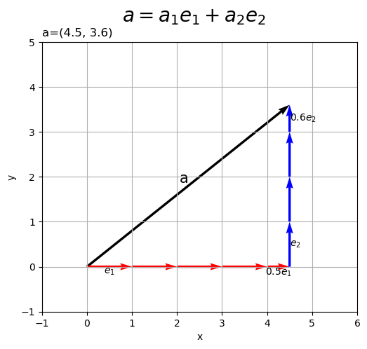
　 $\mathbf{a}$ の各要素 $a_1, a_2$ をスカラー値として、 $a_1$ 個の $\mathbf{e}_1$ と $a_2$ 個の $\mathbf{e}_2$ を描画します(色々対応してたらアレなコードになってしましました)。

　ベクトルの値を変化させたアニメーションを作成します。

・作図コード(クリックで展開)

# フレーム数を設定
frame_num = 51

# 各次元の要素として利用する値を指定
a_vals = np.array(
    [np.linspace(start=-4.0, stop=6.0, num=frame_num), 
     np.linspace(start=-6.4, stop=3.6, num=frame_num)]
).T

# 作図用の値を設定
x_min = np.floor(np.min([0.0, *a_vals[:, 0]])) - 1
x_max = np.ceil(np.max([0.0, *a_vals[:, 0]])) + 1
y_min = np.floor(np.min([0.0, *a_vals[:, 1]])) - 1
y_max = np.ceil(np.max([0.0, *a_vals[:, 1]])) + 1

# 作図用のオブジェクトを初期化
fig, ax = plt.subplots(figsize=(6, 6), facecolor='white')
fig.suptitle('$a = a_1 e_1 + a_2 e_2$', fontsize=20)
    
# 作図処理を関数として定義
def update(i):
    
    # 前フレームのグラフを初期化
    plt.cla()
    
    # i番目のベクトルを取得
    a = a_vals[i].round(5)
    
    # 作図用の値を設定
    sign_x = np.sign(a[0])
    sign_y = np.sign(a[1])
    num_x = int(np.ceil(abs(a[0])))
    num_y = int(np.ceil(abs(a[1])))
    
    # 2Dベクトル差を作図
    ax.quiver(0, 0, *a, angles='xy', scale_units='xy', scale=1) # ベクトルa
    for j in range(num_x):
        if j+1 <= abs(a[0]):
            # x軸方向の単位ベクトルを描画
            ax.quiver(sign_x*j, 0, *sign_x*e1, color='red', 
                      angles='xy', scale_units='xy', scale=1) # ベクトルe1
        else:
            # x軸方向の差分のベクトルを描画
            diff_x = a[0] - sign_x * j
            ax.quiver(sign_x*j, 0, diff_x, e1[1], color='red', 
                      angles='xy', scale_units='xy', scale=1) # ベクトルw1e1
            ax.annotate(xy=[sign_x*i+0.5*diff_x, e1[1]], text='$'+str(diff_x.round(2))+'e_1$', 
                        size=10, ha='center', va='top') # ベクトルw1e1ラベル
    for k in range(num_y):
        if k+1 <= abs(a[1]):
            # y軸方向の単位ベクトルを描画
            ax.quiver(a[0], sign_y*k, *sign_y*e2, color='blue', 
                      angles='xy', scale_units='xy', scale=1) # ベクトルe2
        else:
            # y軸方向の差分のベクトルを描画
            diff_y = a[1] - sign_y * k
            ax.quiver(a[0], sign_y*k, e2[0], diff_y, color='blue', 
                      angles='xy', scale_units='xy', scale=1) # ベクトルw2e2
            ax.annotate(xy=[a[0], sign_y*k+0.5*diff_y], text='$'+str(diff_y.round(2))+'e_2$', 
                        size=10, ha='left', va='center') # ベクトルw2e2ラベル
    ax.annotate(xy=0.5*a, text='a', 
                size=10, ha='right', va='bottom') # ベクトルaラベル
    if abs(a[0]) >= 1.0 or a[0] == 0.0:
        sign_x_str = [sign_str_lt[idx] for idx, bl in enumerate([a[0] >= 1.0, a[0] == 0.0, a[0] <= -1.0]) if bl][0]
        ax.annotate(xy=sign_x*0.5*e1, text='$'+sign_x_str+'e_1$', 
                    size=10, ha='center', va='top') # ベクトルe1ラベル
    if abs(a[1]) >= 1.0 or a[1] == 0.0:
        sign_y_str = [sign_str_lt[idx] for idx, bl in enumerate([a[1] >= 1.0, a[1] == 0.0, a[1] <= -1.0]) if bl][0]
        ax.annotate(xy=[a[0], sign_y*0.5*e2[1]], text='$'+sign_y_str+'e_2$', 
                    size=10, ha='left', va='center') # ベクトルe2ラベル
    ax.set_xticks(ticks=np.arange(x_min, x_max+1))
    ax.set_yticks(ticks=np.arange(y_min, y_max+1))
    ax.grid()
    ax.set_xlabel('x')
    ax.set_ylabel('y')
    ax.set_title('a=('+', '.join(map(str, a.round(2)))+')', loc='left')
    ax.set_aspect('equal')

# gif画像を作成
ani = FuncAnimation(fig=fig, func=update, frames=frame_num, interval=100)

# gif画像を保存
ani.save('linearcomb_unitvector_2d.gif')

　作図処理をupdate()として定義して、FuncAnimation()でgif画像を作成します。

3次元の場合

　続いて、3次元空間上での線形結合を可視化します。

　3次元ベクトルとと標準単位ベクトルを指定します。

# ベクトルを指定
a = np.array([4.5, 3.6, 2.7])

# 係数を指定
e1 = np.array([1.0, 0.0, 0.0])
e2 = np.array([0.0, 1.0, 0.0])
e3 = np.array([0.0, 0.0, 1.0])

　 $\mathbf{a} = (a_1, a_2, a_3)^{\top}$ をa、 $\mathbf{e}_1 = (1, 0, 0)^{\top}, \mathbf{e}_2 = (0, 1, 0)^{\top}$ , $\mathbf{e}_3 = (0, 0, 1)^{\top}$ をe1, e2, e3として値を指定します。

　3次元空間上に4つのベクトル $\mathbf{a}, \mathbf{e}_1, \mathbf{e}_2, \mathbf{e}_3$ を描画します。

# 作図用の値を設定
x_min = np.floor(np.min([0.0, a[0]])) - 1
x_max = np.ceil(np.max([1.0, a[0]])) + 1
y_min = np.floor(np.min([0.0, a[1]])) - 1
y_max = np.ceil(np.max([1.0, a[1]])) + 1
z_min = np.floor(np.min([0.0, a[2]])) - 1
z_max = np.ceil(np.max([1.0, a[2]])) + 1

# (原点からの)3Dベクトルを作図
fig, ax = plt.subplots(subplot_kw={'projection': '3d'}, 
                       figsize=(7, 7), facecolor='white')
ax.quiver(0, 0, 0, *a, arrow_length_ratio=0.05, color='black') # ベクトルa
ax.quiver(0, 0, 0, *e1, arrow_length_ratio=0.2, color='red') # ベクトルe1
ax.quiver(0, 0, 0, *e2, arrow_length_ratio=0.2, color='blue') # ベクトルe2
ax.quiver(0, 0, 0, *e3, arrow_length_ratio=0.2, color='green') # ベクトルe3
ax.text(*0.5*a, s='a', size=15, ha='center', va='bottom') # ベクトルaラベル
ax.text(*0.5*e1, s='$e_1$', size=10, ha='center', va='top') # ベクトルe1ラベル
ax.text(*0.5*e2, s='$e_2$', size=10, ha='right', va='bottom') # ベクトルe2ラベル
ax.text(*0.5*e3, s='$e_3$', size=10, ha='right', va='center') # ベクトルe3ラベル
ax.quiver([0, a[0]], [0, a[1]], [z_min, z_min], 
          [0, 0], [0, 0], [-z_min, a[2]-z_min], 
          color='gray', arrow_length_ratio=0, linestyle=':') # 補助線
ax.set_xticks(ticks=np.arange(x_min, x_max+1))
ax.set_yticks(ticks=np.arange(y_min, y_max+1))
ax.set_zticks(ticks=np.arange(z_min, z_max+1))
ax.set_zlim(z_min, z_max)
ax.set_xlabel('x')
ax.set_ylabel('y')
ax.set_zlabel('z')
ax.set_title('a=('+', '.join(map(str, a))+')', loc='left')
fig.suptitle('$a, e_1, e_2, e_3$', fontsize=20)
ax.set_aspect('equal')
plt.show()

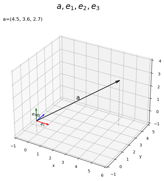
　axes.quiver()の第1・2・3引数に始点の座標、第4・5・6引数にベクトルのサイズを指定します。この例では、原点を始点とします。

　 $a_1 \mathbf{e}_1 + a_2 \mathbf{a}_2 + a_3 \mathbf{a}_3$ のベクトルを描画します。

# 符号を取得
sign_x = np.sign(a[0])
sign_y = np.sign(a[1])
sign_z = np.sign(a[2])

# 単位ベクトルの数を設定
num_x = int(np.ceil(abs(a[0])))
num_y = int(np.ceil(abs(a[1])))
num_z = int(np.ceil(abs(a[2])))

# ラベル用のリストを作成
sign_str_lt = ['', '0', '-']

# 3D標準単位ベクトルの線形結合を作図
fig, ax = plt.subplots(subplot_kw={'projection': '3d'}, 
                       figsize=(7, 7), facecolor='white')
ax.quiver(0, 0, 0, *a, arrow_length_ratio=0.05, color='black') # ベクトルa
for i in range(num_x):
    if i+1 <= abs(a[0]):
        # x軸方向の単位ベクトルを描画
        ax.quiver(sign_x*i, 0, 0, *sign_x*e1, arrow_length_ratio=0.2, color='red') # ベクトルe1
    else:
        # x軸方向の差分のベクトルを描画
        diff_x = a[0] - sign_x * i
        ax.quiver(sign_x*i, 0, 0, diff_x, e1[1], e1[2], arrow_length_ratio=0.2, color='red') # ベクトルw1e1
        ax.text(sign_x*i+0.5*diff_x, e1[1], e1[2], s='$'+str(diff_x.round(2))+'e_1$', 
                size=10, ha='center', va='top') # ベクトルw1e1ラベル
for j in range(num_y):
    if j+1 <= abs(a[1]):
        # y軸方向の単位ベクトルを描画
        ax.quiver(a[0], sign_y*j, 0, *sign_y*e2, arrow_length_ratio=0.2, color='blue') # ベクトルe2
    else:
        # y軸方向の差分のベクトルを描画
        diff_y = a[1] - sign_y * e2[1] * j
        ax.quiver(a[0], sign_y*j, 0, e2[0], diff_y, e2[2], arrow_length_ratio=0.2, color='blue') # ベクトルw2e2
        ax.text(a[0], sign_y*j+0.5*diff_y, e2[2], s='$'+str(diff_y.round(2))+'e_2$', 
                size=10, ha='right', va='bottom') # ベクトルw2e2ラベル
for k in range(num_z):
    if k+1 <= abs(a[2]):
        # z軸方向の単位ベクトルを描画
        ax.quiver(a[0], a[1], sign_z*k, *sign_z*e3, arrow_length_ratio=0.2, color='green') # ベクトルe3
    else:
        # z軸方向の差分のベクトルを描画
        diff_z = a[2] - sign_z * e3[2] * k
        ax.quiver(a[0], a[1], sign_z*k, e3[0], e3[1], diff_z, arrow_length_ratio=0.2, color='green') # ベクトルw2e2
        ax.text(a[0], a[1], sign_z*k+0.5*diff_z, s='$'+str(diff_z.round(2))+'e_3$', 
                size=10, ha='left', va='center') # ベクトルw3e3ラベル
ax.text(*0.5*a, s='a', size=15, ha='center', va='bottom') # ベクトルaラベル
if abs(a[0]) >= 1.0 or a[0] == 0.0:
    sign_x_str = [sign_str_lt[i] for i, b in enumerate([a[0] >= 1.0, a[0] == 0.0, a[0] <= -1.0]) if b][0]
    ax.text(*sign_x*0.5*e1, s='$'+sign_x_str+'e_1$', size=10, ha='center', va='top') # ベクトルe1ラベル
if abs(a[1]) >= 1.0 or a[1] == 0.0:
    sign_y_str = [sign_str_lt[i] for i, b in enumerate([a[1] >= 1.0, a[1] == 0.0, a[1] <= -1.0]) if b][0]
    ax.text(a[0], sign_y*0.5*e2[1], e2[2], s='$'+sign_y_str+'e_2$', size=10, ha='right', va='bottom') # ベクトルe2ラベル
if abs(a[2]) >= 1.0 or a[2] == 0.0:
    sign_z_str = [sign_str_lt[i] for i, b in enumerate([a[2] >= 1.0, a[2] == 0.0, a[2] <= -1.0]) if b][0]
    ax.text(a[0], a[1], sign_z*0.5*e3[2], s='$'+sign_z_str+'e_3$', size=10, ha='left', va='center') # ベクトルe3ラベル
ax.quiver([0, a[0], a[0]], [0, 0, a[1]], [z_min, z_min, z_min], 
          [0, 0, 0], [0, 0, 0], [-z_min, -z_min, -z_min], 
          color='gray', arrow_length_ratio=0, linestyle=':') # 補助線
ax.set_xticks(ticks=np.arange(x_min, x_max+1))
ax.set_yticks(ticks=np.arange(y_min, y_max+1))
ax.set_zticks(ticks=np.arange(z_min, z_max+1))
ax.set_zlim(z_min, z_max)
ax.set_xlabel('x')
ax.set_ylabel('y')
ax.set_zlabel('z')
ax.set_title('a=('+', '.join(map(str, a))+')', loc='left')
fig.suptitle('$a = a_1 e_1 + a_2 e_2 + a_3 e_3$', fontsize=20)
ax.set_aspect('equal')
plt.show()

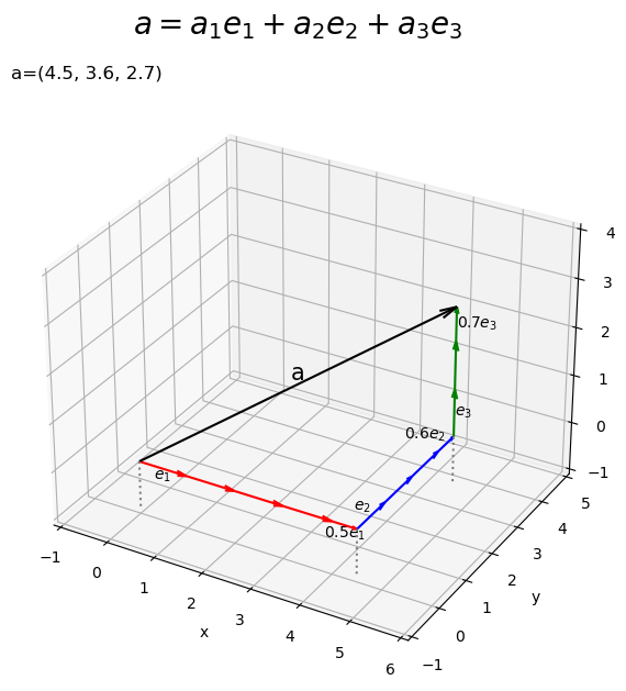
　 $\mathbf{a}$ の各要素 $a_1, a_2, a_3$ をスカラー値として、 $a_1$ 個の $\mathbf{e}_1$ と $a_2$ 個の $\mathbf{e}_2$ と $a_3$ 個の $\mathbf{e}_3$ を描画します(もっと上手く処理できれば教えて下さい)。

　ベクトルの値を変化させたアニメーションを作成します。

・作図コード(クリックで展開)

# フレーム数を設定
frame_num = 51

# 各次元の要素として利用する値を指定
a_vals = np.array(
    [np.linspace(start=-4.0, stop=6.0, num=frame_num), 
     np.linspace(start=-6.4, stop=3.6, num=frame_num), 
     np.linspace(start=-3.0, stop=3.0, num=frame_num)]
).T

# 作図用の値を設定
x_min = np.floor(np.min([0.0, *a_vals[:, 0]])) - 1
x_max = np.ceil(np.max([0.0, *a_vals[:, 0]])) + 1
y_min = np.floor(np.min([0.0, *a_vals[:, 1]])) - 1
y_max = np.ceil(np.max([0.0, *a_vals[:, 1]])) + 1
z_min = np.floor(np.min([0.0, *a_vals[:, 2]])) - 1
z_max = np.ceil(np.max([0.0, *a_vals[:, 2]])) + 1

# 作図用のオブジェクトを初期化
fig, ax = plt.subplots(subplot_kw={'projection': '3d'}, 
                       figsize=(7, 7), facecolor='white')
fig.suptitle('$a = a_1 e_1 + a_2 e_2 + a_3 e_3$', fontsize=20)

# 作図処理を関数として定義
def update(i):
    
    # 前フレームのグラフを初期化
    plt.cla()
    
    # i番目のベクトルを取得
    a = a_vals[i].round(5)
    
    # 作図用の値を設定
    sign_x = np.sign(a[0])
    sign_y = np.sign(a[1])
    sign_z = np.sign(a[2])
    num_x = int(np.ceil(abs(a[0])))
    num_y = int(np.ceil(abs(a[1])))
    num_z = int(np.ceil(abs(a[2])))
    
    # 3D標準単位ベクトルの線形結合を作図
    ax.quiver(0, 0, 0, *a, arrow_length_ratio=0.05, color='black') # ベクトルa
    for j in range(num_x):
        if j+1 <= abs(a[0]):
            # x軸方向の単位ベクトルを描画
            ax.quiver(sign_x*j, 0, 0, *sign_x*e1, arrow_length_ratio=0.2, color='red') # ベクトルe1
        else:
            # x軸方向の差分のベクトルを描画
            diff_x = a[0] - sign_x * j
            ax.quiver(sign_x*j, 0, 0, diff_x, e1[1], e1[2], arrow_length_ratio=0.2, color='red') # ベクトルw1e1
            ax.text(sign_x*j+0.5*diff_x, e1[1], e1[2], s='$'+str(diff_x.round(2))+'e_1$', 
                    size=10, ha='center', va='top') # ベクトルw1e1ラベル
    for k in range(num_y):
        if k+1 <= abs(a[1]):
            # y軸方向の単位ベクトルを描画
            ax.quiver(a[0], sign_y*k, 0, *sign_y*e2, arrow_length_ratio=0.2, color='blue') # ベクトルe2
        else:
            # y軸方向の差分のベクトルを描画
            diff_y = a[1] - sign_y * k
            ax.quiver(a[0], sign_y*k, 0, e2[0], diff_y, e2[2], arrow_length_ratio=0.2, color='blue') # ベクトルw2e2
            ax.text(a[0], sign_y*k+0.5*diff_y, e2[2], s='$'+str(diff_y.round(2))+'e_2$', 
                    size=10, ha='right', va='bottom') # ベクトルw2e2ラベル
    for l in range(num_z):
        if l+1 <= abs(a[2]):
            # z軸方向の単位ベクトルを描画
            ax.quiver(a[0], a[1], sign_z*l, *sign_z*e3, arrow_length_ratio=0.2, color='green') # ベクトルe3
        else:
            # z軸方向の差分のベクトルを描画
            diff_z = a[2] - sign_z * l
            ax.quiver(a[0], a[1], sign_z*l, e3[0], e3[1], diff_z, arrow_length_ratio=0.2, color='green') # ベクトルw2e2
            ax.text(a[0], a[1], sign_z*l+0.5*diff_z, s='$'+str(diff_z.round(2))+'e_3$', 
                    size=10, ha='left', va='center') # ベクトルw3e3ラベル
    ax.text(*0.5*a, s='a', size=10, ha='center', va='bottom') # ベクトルaラベル
    if abs(a[0]) >= 1.0 or a[0] == 0.0:
        sign_x_str = [sign_str_lt[i] for i, b in enumerate([a[0] >= 1.0, a[0] == 0.0, a[0] <= -1.0]) if b][0]
        ax.text(*sign_x*0.5*e1, s='$'+sign_x_str+'e_1$', size=10, ha='center', va='top') # ベクトルe1ラベル
    if abs(a[1]) >= 1.0 or a[1] == 0.0:
        sign_y_str = [sign_str_lt[i] for i, b in enumerate([a[1] >= 1.0, a[1] == 0.0, a[1] <= -1.0]) if b][0]
        ax.text(a[0], sign_y*0.5*e2[1], e2[2], s='$'+sign_y_str+'e_2$', size=10, ha='right', va='bottom') # ベクトルe2ラベル
    if abs(a[2]) >= 1.0 or a[2] == 0.0:
        sign_z_str = [sign_str_lt[i] for i, b in enumerate([a[2] >= 1.0, a[2] == 0.0, a[2] <= -1.0]) if b][0]
        ax.text(a[0], a[1], sign_z*0.5*e3[2], s='$'+sign_z_str+'e_3$', size=10, ha='left', va='center') # ベクトルe3ラベル
    ax.quiver([0, a[0], a[0]], [0, 0, a[1]], [z_min, z_min, z_min], 
              [0, 0, 0], [0, 0, 0], [-z_min, -z_min, -z_min], 
              color='gray', arrow_length_ratio=0, linestyle=':') # 補助線
    ax.set_xticks(ticks=np.arange(x_min, x_max+1))
    ax.set_yticks(ticks=np.arange(y_min, y_max+1))
    ax.set_zticks(ticks=np.arange(z_min, z_max+1))
    ax.set_zlim(z_min, z_max)
    ax.set_xlabel('x')
    ax.set_ylabel('y')
    ax.set_zlabel('z')
    ax.set_title('a=('+', '.join(map(str, a.round(2)))+')', loc='left')
    ax.set_aspect('equal')

# gif画像を作成
ani = FuncAnimation(fig=fig, func=update, frames=frame_num, interval=100)

# gif画像を保存
ani.save('linearcomb_unitvector_3d.gif')

　この記事では、標準単位ベクトルの線形結合を可視化しました。次の記事では、アフィン結合を可視化します。

参考書籍

Stephen Boyd・Lieven Vandenberghe(著),玉木徹(訳)『スタンフォード　ベクトル・行列からはじめる最適化数学』講談社サイエンティク,2021年.

おわりに

　前回がベクトルの線形結合で、今回はそもそもベクトルは標準単位ベクトルの線形結合でできているという話です。
　数式を見ると、ベクトルの各要素を0か1を持つベクトルに掛けて足したら元のベクトルになると言われても、そりゃそうだと思ってしまいますが、標準単位ベクトルが並んでるのを見ればなるほどと思えました。

　そんなグラフを作ろうと試行錯誤してたらおまじない的な処理が増えてしまいました。3日後の自分でも分からないと思うので、読んだ人が分からなくても当然だと思います。
　書き始めの段階に自然数のみで組んでたときはシンプルに実装できたんです。

【次の内容】

からっぽのしょこ

読んだら書く！書いたら読む！同じ事は二度調べ(たく)ない

【Python】1.3：標準単位ベクトルの線形結合の可視化【『スタンフォード線形代数入門』のノート】