はじめに
『スタンフォード ベクトル・行列からはじめる最適化数学』の学習ノートです。
本の内容に関して「Pythonを使って再現」や「数式の行間埋め」によって理解を目指します。本と一緒に読んでください。
この記事は1.2節「ベクトルの和」の内容です。
ベクトルの和を可視化します。
【前の内容】
【他の内容】
【今回の内容】
ベクトルの和の可視化
2つのベクトルの和をグラフで確認します。
ベクトルの作図については「【Python】ベクトルの例【『スタンフォード線形代数入門』のノート】 - からっぽのしょこ」を参照してください。
利用するライブラリを読み込みます。
# 利用ライブラリ
import numpy as np
import matplotlib.pyplot as plt
from matplotlib.animation import FuncAnimation
2次元の場合
まずは、2次元空間(平面)上でベクトルの和を可視化します。
2つの2次元ベクトルを指定します。
# ベクトルを指定
a = np.array([5.0, 1.0])
b = np.array([-1.0, 3.0])
を
a、を
bとして値を指定します。ただし、Pythonでは0からインデックスが割り当てられるので、の値は
a[0]に対応します。
2次元空間(平面)上に2つのベクトルを描画します。
# 作図用の値を設定
x_min = np.floor(np.min([0.0, a[0], b[0]])) - 1
x_max = np.ceil(np.max([0.0, a[0], b[0]])) + 1
y_min = np.floor(np.min([0.0, a[1], b[1]])) - 1
y_max = np.ceil(np.max([0.0, a[1], b[1]])) + 1

# (原点からの)2Dベクトルを作図
fig, ax = plt.subplots(figsize=(6, 4.5), facecolor='white')
ax.quiver(0, 0, *a, color='red', angles='xy', scale_units='xy', scale=1) # ベクトルa
ax.quiver(0, 0, *b, color='blue', angles='xy', scale_units='xy', scale=1) # ベクトルb
ax.annotate(xy=0.5*a, text='a', size=15, ha='center', va='top') # ベクトルaラベル
ax.annotate(xy=0.5*b, text='b', size=15, ha='right', va='center') # ベクトルbラベル
ax.set_xticks(ticks=np.arange(x_min, x_max+1))
ax.set_yticks(ticks=np.arange(y_min, y_max+1))
ax.grid()
ax.set_xlabel('x')
ax.set_ylabel('y')
ax.set_title('a=('+', '.join(map(str, a))+'), ' +
             'b=('+', '.join(map(str, b))+')', loc='left')
fig.suptitle('vector a, b', fontsize=20)
ax.set_aspect('equal')
plt.show()
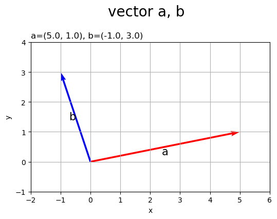
ベクトルのグラフを
axes.quiver()で描画します。第1・2引数に始点の座標、第3・4引数にベクトルのサイズ(変化量)を指定します。この例では、原点を始点とします。
配列a, bの前に*を付けてアンパック(展開)して指定しています。
のベクトルを描画します。
# 作図用の値を設定
x_min = np.floor(np.min([0.0, a[0], b[0], a[0]+b[0]])) - 1
x_max = np.ceil(np.max([0.0, a[0], b[0], a[0]+b[0]])) + 1
y_min = np.floor(np.min([0.0, a[1], b[1], a[1]+b[1]])) - 1
y_max = np.ceil(np.max([0.0, a[1], b[1], a[1]+b[1]])) + 1

# 2Dベクトル和を作図
fig, ax = plt.subplots(figsize=(6, 5), facecolor='white')
ax.quiver(0, 0, *a, color='red', angles='xy', scale_units='xy', scale=1) # ベクトルa
ax.quiver(*b, *a, color='red', angles='xy', scale_units='xy', scale=1) # ベクトルa
ax.quiver(0, 0, *b, color='blue', angles='xy', scale_units='xy', scale=1) # ベクトルb
ax.quiver(*a, *b, color='blue', angles='xy', scale_units='xy', scale=1) # ベクトルb
ax.quiver(0, 0, *a+b, color='purple', angles='xy', scale_units='xy', scale=1) # ベクトルa+b
ax.annotate(xy=0.5*a, text='a', size=15, ha='center', va='top') # ベクトルaラベル
ax.annotate(xy=0.5*b, text='b', size=15, ha='right', va='center') # ベクトルbラベル
ax.annotate(xy=0.5*(a+b), text='a+b', size=15, ha='left', va='top') # ベクトルa+bラベル
ax.annotate(xy=0.5*(b+a), text='b+a', size=15, ha='right', va='bottom') # ベクトルb+aラベル
ax.set_xticks(ticks=np.arange(x_min, x_max+1))
ax.set_yticks(ticks=np.arange(y_min, y_max+1))
ax.grid()
ax.set_xlabel('x')
ax.set_ylabel('y')
ax.set_title('a=('+', '.join(map(str, a))+'), ' +
             'b=('+', '.join(map(str, b))+')', loc='left')
fig.suptitle('vector a+b, b+a', fontsize=20)
ax.set_aspect('equal')
plt.show()

(下の組み合わせ)と
(上の組み合わせ)が一致するのが分かります。
原点と点を重ねて描画します。
# 2Dベクトル和を作図
fig, ax = plt.subplots(figsize=(6, 5), facecolor='white')
ax.quiver(0, 0, *a, color='red', angles='xy', scale_units='xy', scale=1, label='a') # ベクトルa
ax.quiver(*b, *a, color='red', angles='xy', scale_units='xy', scale=1) # ベクトルa
ax.quiver(0, 0, *b, color='blue', angles='xy', scale_units='xy', scale=1, label='b') # ベクトルb
ax.quiver(*a, *b, color='blue', angles='xy', scale_units='xy', scale=1) # ベクトルb
ax.quiver(0, 0, *a+b, color='purple', angles='xy', scale_units='xy', scale=1, label='a+b') # ベクトルa+b
ax.scatter(0, 0, c='orange', s=100) # 原点
ax.scatter(*a, c='red', s=100) # 点a
ax.scatter(*b, c='blue', s=100) # 点b
ax.scatter(*a+b, c='purple', s=100) # 点a+b
ax.annotate(xy=[0, 0], text='O', size=15, ha='right', va='top') # 原点ラベル
ax.annotate(xy=a, text='a', size=15, ha='left', va='top') # 点aラベル
ax.annotate(xy=b, text='b', size=15, ha='right', va='bottom') # 点bラベル
ax.annotate(xy=a+b, text='a+b', size=15, ha='center', va='bottom') # 点a+bラベル
ax.set_xticks(ticks=np.arange(x_min, x_max+1))
ax.set_yticks(ticks=np.arange(y_min, y_max+1))
ax.grid()
ax.set_xlabel('x')
ax.set_ylabel('y')
ax.set_title('a=('+', '.join(map(str, a))+'), ' +
             'b=('+', '.join(map(str, b))+')', loc='left')
fig.suptitle('point a, b, a+b', fontsize=20)
ax.legend()
ax.set_aspect('equal')
plt.show()
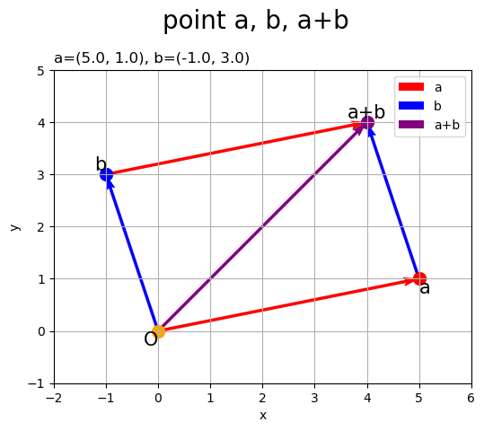
点から
移動した点は
、点
から
移動した点も
になるのが分かります。
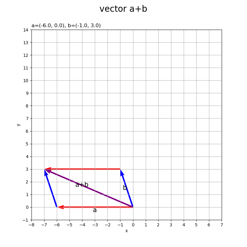
ベクトルの値を変化させたアニメーションを作成します。
・作図コード(クリックで展開)
# フレーム数を設定
frame_num = 51

# 各次元の要素として利用する値を指定
a_vals = np.array(
    [np.linspace(start=-6.0, stop=6.0, num=frame_num),
     np.linspace(start=0.0, stop=10.0, num=frame_num)]
).T
b_vals = np.array(
    [np.linspace(start=-1.0, stop=-1.0, num=frame_num),
     np.linspace(start=3.0, stop=3.0, num=frame_num)]
).T

# 作図用の値を設定
x_min = np.floor(np.min([0.0, *a_vals[:, 0], *b_vals[:, 0], *a_vals[:, 0]+b_vals[:,0]])) - 1
x_max = np.ceil(np.max([0.0, *a_vals[:, 0], *b_vals[:, 0], *a_vals[:, 0]+b_vals[:, 0]])) + 1
y_min = np.floor(np.min([0.0, *a_vals[:, 1], *b_vals[:, 1], *a_vals[:, 1]+b_vals[:, 1]])) - 1
y_max = np.ceil(np.max([0.0, *a_vals[:, 1], *b_vals[:, 1], *a_vals[:, 1]+b_vals[:, 1]])) + 1

# 作図用のオブジェクトを初期化
fig, ax = plt.subplots(figsize=(8, 8), facecolor='white')
fig.suptitle('vector a+b', fontsize=20)

# 作図処理を関数として定義
def update(i):

    # 前フレームのグラフを初期化
    plt.cla()

    # i番目のベクトルを作成
    a = a_vals[i]
    b = b_vals[i]

    # 2Dベクトル和を作図
    ax.quiver(0, 0, *a, color='red', angles='xy', scale_units='xy', scale=1) # ベクトルa
    ax.quiver(*b, *a, color='red', angles='xy', scale_units='xy', scale=1) # ベクトルa
    ax.quiver(0, 0, *b, color='blue', angles='xy', scale_units='xy', scale=1) # ベクトルb
    ax.quiver(*a, *b, color='blue', angles='xy', scale_units='xy', scale=1) # ベクトルb
    ax.quiver(0, 0, *a+b, color='purple', angles='xy', scale_units='xy', scale=1) # ベクトルa+b
    ax.annotate(xy=0.5*a, text='a', size=15, ha='center', va='top') # ベクトルaラベル
    ax.annotate(xy=0.5*b, text='b', size=15, ha='right', va='center') # ベクトルbラベル
    ax.annotate(xy=0.5*(a+b), text='a+b', size=15, ha='right', va='bottom') # ベクトルa+bラベル
    ax.set_xticks(ticks=np.arange(x_min, x_max+1))
    ax.set_yticks(ticks=np.arange(y_min, y_max+1))
    ax.grid()
    ax.set_xlabel('x')
    ax.set_ylabel('y')
    ax.set_title('a=('+', '.join(map(str, a.round(2)))+'), ' +
                 'b=('+', '.join(map(str, b.round(2)))+')', loc='left')
    ax.set_aspect('equal')

# gif画像を作成
ani = FuncAnimation(fig=fig, func=update, frames=frame_num, interval=100)

# gif画像を保存
ani.save('sum_vector_2d.gif')
作図処理をupdate()として定義して、FuncAnimation()でgif画像を作成します。
3次元の場合
続いて、3次元空間上でベクトルの和を可視化します。
3次元ベクトルを指定します。
# ベクトルを指定
a = np.array([5.0, 1.0, 3.0])
b = np.array([-1.0, 3.0, 2.0])
を
a、を
bとして値を指定します。
3次元空間上に2つのベクトルを描画します。
# 作図用の値を設定
x_min = np.floor(np.min([0.0, a[0], b[0]])) - 1
x_max = np.ceil(np.max([0.0, a[0], b[0]])) + 1
y_min = np.floor(np.min([0.0, a[1], b[1]])) - 1
y_max = np.ceil(np.max([0.0, a[1], b[1]])) + 1
z_min = np.floor(np.min([0.0, a[2], b[2]])) - 1
z_max = np.ceil(np.max([0.0, a[2], b[2]])) + 1

# (原点からの)3Dベクトルを作図
fig, ax = plt.subplots(figsize=(8, 8), subplot_kw={'projection': '3d'}, facecolor='white')
ax.quiver(0, 0, 0, *a, color='red', arrow_length_ratio=0.05) # ベクトルa
ax.quiver(0, 0, 0, *b, color='blue', arrow_length_ratio=0.05) # ベクトルb
ax.text(*0.5*a, s='a', size=15, ha='center', va='top') # ベクトルaラベル
ax.text(*0.5*b, s='b', size=15, ha='right', va='center') # ベクトルbラベル
ax.quiver([0, a[0], b[0]], [0, a[1], b[1]], [z_min, z_min, z_min],
          [0, 0, 0], [0, 0, 0], [-z_min, a[2]-z_min, b[2]-z_min],
          color='gray', arrow_length_ratio=0, linestyle=':') # 補助線
ax.set_xticks(ticks=np.arange(x_min, x_max+1))
ax.set_yticks(ticks=np.arange(y_min, y_max+1))
ax.set_zticks(ticks=np.arange(z_min, z_max+1))
ax.set_zlim(z_min, z_max)
ax.set_xlabel('x')
ax.set_ylabel('y')
ax.set_zlabel('z')
ax.set_title('a=('+', '.join(map(str, a))+'), ' +
             'b=('+', '.join(map(str, b))+')', loc='left')
fig.suptitle('vector a, b', fontsize=20)
ax.set_aspect('equal')
plt.show()
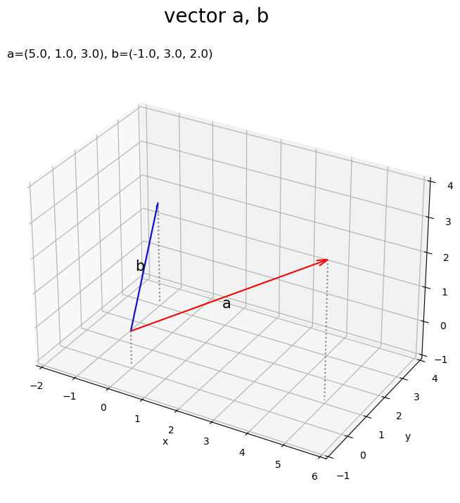
axes.quiver()の第1・2・3引数に始点の座標、第4・5・6引数にベクトルのサイズを指定します。この例では、原点を始点とします。
のベクトルを描画します。
# 作図用の値を設定
x_min = np.floor(np.min([0.0, a[0], b[0], a[0]+b[0]])) - 1
x_max = np.ceil(np.max([0.0, a[0], b[0], a[0]+b[0]])) + 1
y_min = np.floor(np.min([0.0, a[1], b[1], a[1]+b[1]])) - 1
y_max = np.ceil(np.max([0.0, a[1], b[1], a[1]+b[1]])) + 1
z_min = np.floor(np.min([0.0, a[2], b[2], a[2]+b[2]])) - 1
z_max = np.ceil(np.max([0.0, a[2], b[2], a[2]+b[2]])) + 1

# 3Dベクトル和を作図
fig, ax = plt.subplots(figsize=(8, 8), subplot_kw={'projection': '3d'}, facecolor='white')
ax.quiver(0, 0, 0, *a, color='red', arrow_length_ratio=0.05) # ベクトルa
ax.quiver(*b, *a, color='red', arrow_length_ratio=0.05) # ベクトルa
ax.quiver(0, 0, 0, *b, color='blue', arrow_length_ratio=0.05) # ベクトルb
ax.quiver(*a, *b, color='blue', arrow_length_ratio=0.05) # ベクトルb
ax.quiver(0, 0, 0, *a+b, color='purple', arrow_length_ratio=0.05) # ベクトルa+b
ax.text(*0.5*a, s='a', size=15, ha='center', va='top') # ベクトルaラベル
ax.text(*0.5*b, s='b', size=15, ha='right', va='center') # ベクトルbラベル
ax.text(*0.5*(a+b), s='a+b', size=15, ha='left', va='top') # ベクトルa+bラベル
ax.text(*0.5*(b+a), s='b+a', size=15, ha='right', va='bottom') # ベクトルb+aラベル
ax.quiver([0, a[0], b[0], a[0]+b[0]], [0, a[1], b[1], a[1]+b[1]], [z_min, z_min, z_min, z_min],
          [0, 0, 0, 0], [0, 0, 0, 0], [-z_min, a[2]-z_min, b[2]-z_min, a[2]+b[2]-z_min],
          color='gray', arrow_length_ratio=0, linestyle=':') # 補助線
ax.set_xticks(ticks=np.arange(x_min, x_max+1))
ax.set_yticks(ticks=np.arange(y_min, y_max+1))
ax.set_zticks(ticks=np.arange(z_min, z_max+1))
ax.set_zlim(z_min, z_max)
ax.set_xlabel('x')
ax.set_ylabel('y')
ax.set_zlabel('z')
ax.set_title('a=('+', '.join(map(str, a))+'), ' +
             'b=('+', '.join(map(str, b))+')', loc='left')
fig.suptitle('vector a+b, b+a', fontsize=20)
ax.set_aspect('equal')
plt.show()
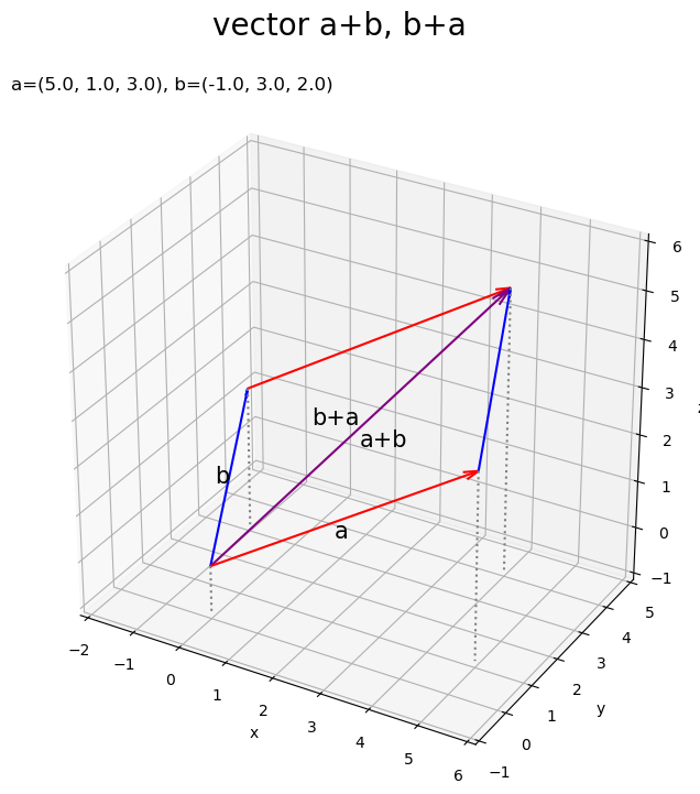
3次元の場合もとなるのが分かります。
原点と点を重ねて描画します。
# 作図用の値を設定
x_min = np.floor(np.min([0.0, a[0], b[0], a[0]+b[0]])) - 1
x_max = np.ceil(np.max([0.0, a[0], b[0], a[0]+b[0]])) + 1
y_min = np.floor(np.min([0.0, a[1], b[1], a[1]+b[1]])) - 1
y_max = np.ceil(np.max([0.0, a[1], b[1], a[1]+b[1]])) + 1
z_min = np.floor(np.min([0.0, a[2], b[2], a[2]+b[2]])) - 1
z_max = np.ceil(np.max([0.0, a[2], b[2], a[2]+b[2]])) + 1

# 3Dベクトル和を作図
fig, ax = plt.subplots(figsize=(8, 8), subplot_kw={'projection': '3d'}, facecolor='white')
ax.quiver(0, 0, 0, *a, color='red', arrow_length_ratio=0.05, label='a') # ベクトルa
ax.quiver(*b, *a, color='red', arrow_length_ratio=0.05) # ベクトルa
ax.quiver(0, 0, 0, *b, color='blue', arrow_length_ratio=0.05, label='b') # ベクトルb
ax.quiver(*a, *b, color='blue', arrow_length_ratio=0.05) # ベクトルb
ax.quiver(0, 0, 0, *a+b, color='purple', arrow_length_ratio=0.05, label='a+b') # ベクトルa+b
ax.scatter(0, 0, 0, c='orange', s=100) # 原点
ax.scatter(*a, c='red', s=100) # 点a
ax.scatter(*b, c='blue', s=100) # 点b
ax.scatter(*a+b, c='purple', s=100) # 点a+b
ax.text(0, 0, 0, s='O', size=15, ha='center', va='top', zorder=20) # 原点ラベル
ax.text(*a, s='a', size=15, ha='center', va='top', zorder=20) # 点aラベル
ax.text(*b, s='b', size=15, ha='right', va='center', zorder=20) # 点bラベル
ax.text(*a+b, s='a+b', size=15, ha='right', va='bottom', zorder=20) # 点bラベル
ax.quiver([0, a[0], b[0], a[0]+b[0]],
          [0, a[1], b[1], a[1]+b[1]],
          [z_min, z_min, z_min, z_min],
          [0, 0, 0, 0],
          [0, 0, 0, 0],
          [-z_min, a[2]-z_min, b[2]-z_min, a[2]+b[2]-z_min],
          color='gray', arrow_length_ratio=0, linestyle=':') # 補助線
ax.set_xticks(ticks=np.arange(x_min, x_max+1))
ax.set_yticks(ticks=np.arange(y_min, y_max+1))
ax.set_zticks(ticks=np.arange(z_min, z_max+1))
ax.set_zlim(z_min, z_max)
ax.set_xlabel('x')
ax.set_ylabel('y')
ax.set_zlabel('z')
ax.set_title('a=('+', '.join(map(str, a))+'), ' +
             'b=('+', '.join(map(str, b))+')', loc='left')
fig.suptitle('point a, b, a+b', fontsize=20)
ax.legend()
ax.set_aspect('equal')
plt.show()
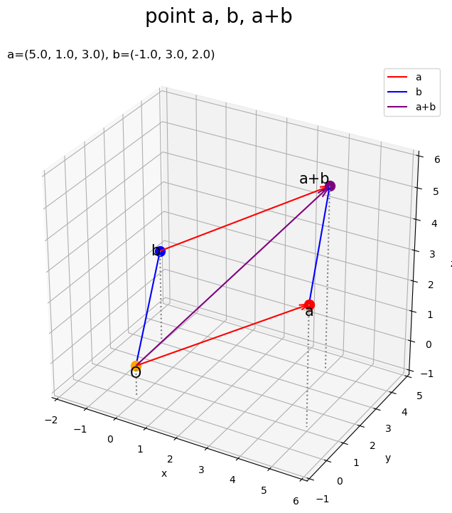
3次元でも、点から
移動した点、点
から
移動した点が
になるのが分かります。
ベクトルの値を変化させたアニメーションを作成します。
・作図コード(クリックで展開)
# フレーム数を設定
frame_num = 51

# 各次元の要素として利用する値を指定
a_vals = np.array(
    [np.linspace(start=-6.0, stop=6.0, num=frame_num),
     np.linspace(start=0.0, stop=10.0, num=frame_num),
     np.linspace(start=-2.0, stop=3.0, num=frame_num)]
).T
b_vals = np.array(
    [np.linspace(start=-1.0, stop=-1.0, num=frame_num),
     np.linspace(start=3.0, stop=3.0, num=frame_num),
     np.linspace(start=2.0, stop=2.0, num=frame_num)]
).T

# 作図用の値を設定
x_min = np.floor(np.min([0.0, *a_vals[:, 0], *b_vals[:, 0], *a_vals[:, 0]+b_vals[:,0]])) - 1
x_max = np.ceil(np.max([0.0, *a_vals[:, 0], *b_vals[:, 0], *a_vals[:, 0]+b_vals[:, 0]])) + 1
y_min = np.floor(np.min([0.0, *a_vals[:, 1], *b_vals[:, 1], *a_vals[:, 1]+b_vals[:, 1]])) - 1
y_max = np.ceil(np.max([0.0, *a_vals[:, 1], *b_vals[:, 1], *a_vals[:, 1]+b_vals[:, 1]])) + 1
z_min = np.floor(np.min([0.0, *a_vals[:, 2], *b_vals[:, 2], *a_vals[:, 2]+b_vals[:, 1]])) - 1
z_max = np.ceil(np.max([0.0, *a_vals[:, 2], *b_vals[:, 2], *a_vals[:, 2]+b_vals[:, 1]])) + 1

# 作図用のオブジェクトを初期化
fig, ax = plt.subplots(figsize=(8, 8), subplot_kw={'projection': '3d'}, facecolor='white')
fig.suptitle('vector a+b', fontsize=20)

# 作図処理を関数として定義
def update(i):

    # 前フレームのグラフを初期化
    plt.cla()

    # i番目のベクトルを作成
    a = a_vals[i]
    b = b_vals[i]

    # 3Dベクトル和を作図
    ax.quiver(0, 0, 0, *a, color='red', arrow_length_ratio=0.05) # ベクトルa
    ax.quiver(*b, *a, color='red', arrow_length_ratio=0.05) # ベクトルa
    ax.quiver(0, 0, 0, *b, color='blue', arrow_length_ratio=0.05) # ベクトルb
    ax.quiver(*a, *b, color='blue', arrow_length_ratio=0.05) # ベクトルb
    ax.quiver(0, 0, 0, *a+b, color='purple', arrow_length_ratio=0.05) # ベクトルa+b
    ax.text(*0.5*a, s='a', size=15, ha='center', va='top') # ベクトルaラベル
    ax.text(*0.5*b, s='b', size=15, ha='right', va='center') # ベクトルbラベル
    ax.text(*0.5*(a+b), s='a+b', size=15, ha='right', va='bottom') # ベクトルb+aラベル
    ax.quiver([0, a[0], b[0], a[0]+b[0]],
              [0, a[1], b[1], a[1]+b[1]],
              [z_min, z_min, z_min, z_min],
              [0, 0, 0, 0],
              [0, 0, 0, 0],
              [-z_min, a[2]-z_min, b[2]-z_min, a[2]+b[2]-z_min],
              color='gray', arrow_length_ratio=0, linestyle=':') # 補助線
    ax.set_xticks(ticks=np.arange(x_min, x_max+1))
    ax.set_yticks(ticks=np.arange(y_min, y_max+1))
    ax.set_zticks(ticks=np.arange(z_min, z_max+1))
    ax.set_zlim(z_min, z_max)
    ax.set_xlabel('x')
    ax.set_ylabel('y')
    ax.set_zlabel('z')
    ax.set_title('a=('+', '.join(map(str, a.round(2)))+'), ' +
                 'b=('+', '.join(map(str, b.round(2)))+')', loc='left')
    ax.set_aspect('equal')

# gif画像を作成
ani = FuncAnimation(fig=fig, func=update, frames=frame_num, interval=100)

# gif画像を保存
ani.save('sum_vector_3d.gif')

この記事では、ベクトルの和を可視化しました。次の記事では、ベクトルの差を可視化します。
参考書籍
- Stephen Boyd・Lieven Vandenberghe(著),玉木 徹(訳)『スタンフォード ベクトル・行列からはじめる最適化数学』講談社サイエンティク,2021年.
おわりに
新しいシリーズの書き始めはいつもレベル感とか一記事の粒度とかノリで悩みます。
投稿日前日に公開された新曲をどうぞ
オケがいる!
【次の内容】