はじめに
R言語で三角関数の定義や公式を可視化しようシリーズです。
この記事では、2つの角の和に関する三角関数の加法定理のグラフを作成します。
【他の記事一覧】
【この記事の内容】
三角関数の加法定の可視化:その1(2角の和)
三角関数における加法定理(2つの角の和のサインとコサイン)をグラフで可視化します。
利用するパッケージを読み込みます。
# 利用パッケージ
library(tidyverse)
library(gganimate)
この記事では、基本的にパッケージ名::関数名()の記法を使うので、パッケージを読み込む必要はありません。ただし、作図コードがごちゃごちゃしないようにパッケージ名を省略しているためggplot2を読み込む必要があります。
また、ネイティブパイプ演算子|>を使っています。magrittrパッケージのパイプ演算子%>%に置き換えても処理できますが、その場合はmagrittrも読み込む必要があります。
加法定理の公式
三角関数の加法定理として、次の関係が成り立ちます。
この記事では、$\sin(\alpha + \beta)$と$\cos(\alpha + \beta)$の式に関して可視化して確認します。
加法定理の可視化
三角関数の加法定理($\sin(\alpha + \beta), \cos(\alpha + \beta)$)をグラフで確認します。
グラフの作成
まずは、角度を固定したグラフを作成します。
角度を指定して、ラジアンに変換します。
# 角度を指定
a <- 30
b <- 45

# ラジアンに変換
alpha <- a / 180 * pi
beta  <- b / 180 * pi
alpha; beta
## [1] 0.5235988
## [1] 0.7853982
度数法における角度$0^{\circ} \leq a \leq 90^{\circ}$、$0^{\circ} \leq b \leq 90^{\circ}$、$a + b \leq 90^{\circ}$を指定します。
指定した角度を、弧度法におけるラジアン$\alpha = a \frac{2 \pi}{360}$、$\beta = b \frac{2 \pi}{360}$に変換します。$\pi$は円周率でpiで扱えます。
・コード(クリックで展開)
(第1象限における)単位円を描画するためのデータフレームを作成します。
# 単位円(の4分の1)の描画用
sector_df <- tibble::tibble(
  c = seq(from = 0, to = 90, by = 1),
  theta = c / 180 * pi,
  x = cos(theta),
  y = sin(theta)
)
sector_df
## # A tibble: 91 × 4
##        c  theta     x      y
##    <dbl>  <dbl> <dbl>  <dbl>
##  1     0 0      1     0
##  2     1 0.0175 1.00  0.0175
##  3     2 0.0349 0.999 0.0349
##  4     3 0.0524 0.999 0.0523
##  5     4 0.0698 0.998 0.0698
##  6     5 0.0873 0.996 0.0872
##  7     6 0.105  0.995 0.105
##  8     7 0.122  0.993 0.122
##  9     8 0.140  0.990 0.139
## 10     9 0.157  0.988 0.156
## # … with 81 more rows
作図用の角度$0^{\circ} \leq c \leq 90^{\circ}$を作成して、ラジアン$\theta = c \frac{2 \pi}{360}$に変換します。
x軸の値は$x = \cos \theta$、y軸の値は$y = \sin \theta$で単位円を描くための点の座標を計算します。
単位正方形を描画するためのデータフレームを作成します。
# 単位正方形の描画用
square_df <- tibble::tibble(
  x = c(0, 0, 1, 1, 0),
  y = c(0, 1, 1, 0, 0)
)
square_df
## # A tibble: 5 × 2
##       x     y
##   <dbl> <dbl>
## 1     0     0
## 2     0     1
## 3     1     1
## 4     1     0
## 5     0     0
単位正方形の頂点の座標を格納します。
加法定理を構成する辺(線分)を描画するためのデータフレームを作成します。
# 因子レベルを指定
fnc_level <- c(
  "1", "sin(a)", "cos(a)",
  "sin(a) cos(b)", "cos(a) sin(b)",
  "sin(a) sin(b)", "cos(a) cos(b)",
  "sin(a+b)", "cos(a+b)"
)

# 辺の描画用
segment_df <- tibble::tribble(
  ~fnc,            ~type,    ~x_from,              ~y_from,              ~x_to,                ~y_to,
  "1",             "main",   0,                    0,                    cos(alpha+beta),      sin(alpha+beta),
  "sin(a)",        "main",   cos(alpha)*cos(beta), cos(alpha)*sin(beta), cos(alpha+beta),      sin(alpha+beta),
  "cos(a)",        "main",   0,                    0,                    cos(alpha)*cos(beta), cos(alpha)*sin(beta),
  "cos(a)",        "sub",    cos(alpha)*cos(beta), cos(alpha)*sin(beta), cos(beta),            sin(beta),
  "sin(a) cos(b)", "main",   cos(alpha)*cos(beta), cos(alpha)*sin(beta), cos(alpha)*cos(beta), sin(alpha+beta),
  "cos(a) sin(b)", "main",   cos(alpha)*cos(beta), 0,                    cos(alpha)*cos(beta), cos(alpha)*sin(beta),
  "sin(a) sin(b)", "main",   cos(alpha+beta),      sin(alpha+beta),      cos(alpha)*cos(beta), sin(alpha+beta),
  "cos(a) cos(b)", "main",   0,                    0,                    cos(alpha)*cos(beta), 0,
  "sin(a+b)",      "target", cos(alpha+beta),      0,                    cos(alpha+beta),      sin(alpha+beta),
  "cos(a+b)",      "target", 0,                    0,                    cos(alpha+beta),      0
) |> # 座標を格納
  dplyr::mutate(
    fnc = factor(fnc, levels = fnc_level) # 因子レベルを設定
  ) |>
  dplyr::arrange(fnc) # 並びを統一
segment_df
## # A tibble: 10 × 6
##    fnc           type   x_from y_from  x_to  y_to
##    <fct>         <chr>   <dbl>  <dbl> <dbl> <dbl>
##  1 1             main    0      0     0.259 0.966
##  2 sin(a)        main    0.612  0.612 0.259 0.966
##  3 cos(a)        main    0      0     0.612 0.612
##  4 cos(a)        sub     0.612  0.612 0.707 0.707
##  5 sin(a) cos(b) main    0.612  0.612 0.612 0.966
##  6 cos(a) sin(b) main    0.612  0     0.612 0.612
##  7 sin(a) sin(b) main    0.259  0.966 0.612 0.966
##  8 cos(a) cos(b) main    0      0     0.612 0
##  9 sin(a+b)      target  0.259  0     0.259 0.966
## 10 cos(a+b)      target  0      0     0.259 0
各辺の値を格納しやすいように、tribble()を使ってデータフレームを作成します。線分の始点の座標をx_from, y_from列、終点の座標をx_to, y_to列とします。次の「関数名ラベル」の関数の値は線分の長さであり、座標の値とは異なります。
各関数(辺)を区別するためのfnc列、「加法定理を示す線("target)」・「加法定理を求めるための線("main)」・「補助線("sub)」を区別するためのtype列を作成します。fnc列は色分け、type列は線の装飾に使います。
線の描画順(重なり順)や色付け順は、fnc列の因子レベルに依存するので、fnc_levelとして指定しておきます。
線分ごとに関数名ラベルを描画するためのデータフレームを作成します。
# 関数名ラベルの描画用
segment_label_df <- segment_df |>
  dplyr::filter(type %in% c("main", "target")) |> # 補助線を除去
  dplyr::group_by(fnc) |> # 中点の計算用
  dplyr::mutate(
    # 線分の中点に配置
    x = median(c(x_from, x_to)),
    y = median(c(y_from, y_to))
  ) |>
  dplyr::ungroup() |>
  dplyr::select(fnc, x, y) |>
  tibble::add_column(
    # ラベルが重ならないように調整
    h = c(1.0, 1.0, 0.5, 0.0, 0.0, 0.5, 0.5, 0.5, 0.5),
    v = c(0.5, 0.5, 0.5, 0.5, 0.5, 0.0, 0.0, 0.5, 1.0),
    # ラベルを作成
    fnc_label = c(
      "1",
      paste0("sin~alpha==", round(sin(alpha), digits = 2)),
      paste0("cos~alpha==", round(cos(alpha), digits = 2)),
      paste0("sin~alpha ~ cos~beta==", round(sin(alpha)*cos(beta), digits = 2)),
      paste0("cos~alpha ~ sin~beta==", round(cos(alpha)*sin(beta), digits = 2)),
      paste0("sin~alpha ~ sin~beta==", round(sin(alpha)*sin(beta), digits = 2)),
      paste0("cos~alpha ~ cos~beta==", round(cos(alpha)*cos(beta), digits = 2)),
      paste0("sin~(alpha+beta)==", round(sin(alpha+beta), digits = 2)),
      paste0("cos~(alpha+beta)==", round(cos(alpha+beta), digits = 2))
    )
  )
segment_label_df
## # A tibble: 9 × 6
##   fnc               x     y     h     v fnc_label
##   <fct>         <dbl> <dbl> <dbl> <dbl> <chr>
## 1 1             0.129 0.483   1     0.5 1
## 2 sin(a)        0.436 0.789   1     0.5 sin~alpha==0.5
## 3 cos(a)        0.306 0.306   0.5   0.5 cos~alpha==0.87
## 4 sin(a) cos(b) 0.612 0.789   0     0.5 sin~alpha ~ cos~beta==0.35
## 5 cos(a) sin(b) 0.612 0.306   0     0.5 cos~alpha ~ sin~beta==0.61
## 6 sin(a) sin(b) 0.436 0.966   0.5   0   sin~alpha ~ sin~beta==0.35
## 7 cos(a) cos(b) 0.306 0       0.5   0   cos~alpha ~ cos~beta==0.61
## 8 sin(a+b)      0.259 0.483   0.5   0.5 sin~(alpha+beta)==0.97
## 9 cos(a+b)      0.129 0       0.5   1   cos~(alpha+beta)==0.26
補助線を取り除いて、各線分の中点にラベルを配置することにします。
辺ごとに(fnc列でグループ化して)、x軸の値はx_from, x_to列、y軸の値はy_from, y_to列の中央値を計算します。
ラベルとして数式を表示するにはexpression()の記法を使います。
直角を示すためのデータフレームを作成します。
# 直角マークの描画用
d <- 0.05
right_angle_df <- tibble::tibble(
  x = c(
    cos(alpha+beta), cos(alpha+beta)-d, cos(alpha+beta)-d,
    cos(alpha)*cos(beta), cos(alpha)*cos(beta)-d, cos(alpha)*cos(beta)-d,
    cos(alpha)*cos(beta)-d, cos(alpha)*cos(beta)-d, cos(alpha)*cos(beta),
    cos(alpha)*cos(beta) + c(cos(beta+0.5*pi)*d, cos(beta+0.5*pi)*d+cos(beta+pi)*d, cos(beta+pi)*d)
  ),
  y = c(
    d, d, 0,
    d, d, 0,
    sin(alpha+beta), sin(alpha+beta)-d, sin(alpha+beta)-d,
    cos(alpha)*sin(beta) + c(sin(beta+0.5*pi)*d, sin(beta+0.5*pi)*d+sin(beta+pi)*d, sin(beta+pi)*d)
  ),
  group = rep(1:4, each = 3) # 角ラベル
)
right_angle_df
## # A tibble: 12 × 3
##        x     y group
##    <dbl> <dbl> <int>
##  1 0.259 0.05      1
##  2 0.209 0.05      1
##  3 0.209 0         1
##  4 0.612 0.05      2
##  5 0.562 0.05      2
##  6 0.562 0         2
##  7 0.562 0.966     3
##  8 0.562 0.916     3
##  9 0.612 0.916     3
## 10 0.577 0.648     4
## 11 0.542 0.612     4
## 12 0.577 0.577     4
直角マークの頂点の座標を計算して格納します。
鋭角を示すためのデータフレームを作成します。
# 角度マーク(扇形)の描画用
d <- 0.09
angle_df <- tibble::tibble(
  # 原点を中心としたときの角度
  c = c(
    seq(from = 0, to = b, by = 1),
    seq(from = b, to = a+b, by = 1),
    seq(from = 90, to = 90+b, by = 1),
    seq(from = 180+b, to = 270, by = 1)
  ), # 角度
  theta = c / 180 * pi, # ラジアン
  group = c(
    rep("b1", times = length(seq(from = 0, to = b, by = 1))),
    rep("a", times = length(seq(from = b, to = a+b, by = 1))),
    rep("b2", times = length(seq(from = 90, to = 90+b, by = 1))),
    rep("90-b", times = length(seq(from = 180+b, to = 270, by = 1)))
  ) |> # 角ラベル
    factor(levels = c("b1", "a", "b2", "90-b")), # 因子レベルを設定
  # 原点を中心としたときの座標
  x = cos(theta) * d,
  y = sin(theta) * d
) |>
  dplyr::mutate(
    # 角ごとに配置
    x = x + c(
      rep(0, times = length(seq(from = 0, to = b, by = 1))),
      rep(0, times = length(seq(from = b, to = a+b, by = 1))),
      rep(cos(alpha)*cos(beta), times = length(seq(from = 90, to = 90+b, by = 1))),
      rep(cos(alpha)*cos(beta), times = length(seq(from = 180+b, to = 270, by = 1)))
    ),
    y = y + c(
      rep(0, times = length(seq(from = 0, to = b, by = 1))),
      rep(0, times = length(seq(from = b, to = a+b, by = 1))),
      rep(cos(alpha)*sin(beta), times = length(seq(from = 90, to = 90+b, by = 1))),
      rep(cos(alpha)*sin(beta), times = length(seq(from = 180+b, to = 270, by = 1)))
    )
  )
angle_df
## # A tibble: 169 × 5
##        c  theta group      x       y
##    <dbl>  <dbl> <fct>  <dbl>   <dbl>
##  1     0 0      b1    0.09   0
##  2     1 0.0175 b1    0.0900 0.00157
##  3     2 0.0349 b1    0.0899 0.00314
##  4     3 0.0524 b1    0.0899 0.00471
##  5     4 0.0698 b1    0.0898 0.00628
##  6     5 0.0873 b1    0.0897 0.00784
##  7     6 0.105  b1    0.0895 0.00941
##  8     7 0.122  b1    0.0893 0.0110
##  9     8 0.140  b1    0.0891 0.0125
## 10     9 0.157  b1    0.0889 0.0141
## # … with 159 more rows
4つの扇形(角度マーク)を描画するための点の角度$0^{\circ} \leq c \leq a + b$、$90^{\circ} \leq c \leq 90^{\circ} + b$、$180^{\circ} + b \leq c \leq 270^{\circ}$を作成して、それぞれラジアン$\theta = c \frac{2 \pi}{360}$に変換して、$x = \cos \theta, y = \sin \theta$で原点を頂点(円の中心)としたときの座標に変換し、角ごとに頂点の座標を加えてプロット位置を変更します。
dはサイズ調整用の値です。
角度ラベルを描画するためのデータフレームを作成します。
# 角度ラベルの描画用
d <- 0.11
angle_label_df <- angle_df |>
  dplyr::group_by(group) |> # 中点の計算用
  dplyr::summarise(
    # 角度の中点に配置
    c = median(c), .groups = "drop"
  ) |>
  dplyr::mutate(
    # 原点を中心としたときの角度
    theta = c / 180 * pi,
    label = c("beta", "alpha", "beta", "90*degree-beta"), # 角ラベル
    # 原点を中心としたときの座標
    x = cos(theta) * d,
    y = sin(theta) * d,
    # 角ごとに配置
    x = x + c(0, 0, cos(alpha)*cos(beta), cos(alpha)*cos(beta)),
    y = y + c(0, 0, cos(alpha)*sin(beta), cos(alpha)*sin(beta))
  )
angle_label_df
## # A tibble: 4 × 6
##   group     c theta label              x      y
##   <fct> <dbl> <dbl> <chr>          <dbl>  <dbl>
## 1 b1     22.5 0.393 beta           0.102 0.0421
## 2 a      60   1.05  alpha          0.055 0.0953
## 3 b2    112.  1.96  beta           0.570 0.714
## 4 90-b  248.  4.32  90*degree-beta 0.570 0.511
角ごとに角度の中点に配置することにします。
角ごとに(group列でグループ化して)、summarise()を使って角度の中央値を計算して、それぞれ座標を計算します。
加法定理の可視化グラフを作成します。
# タイトル用のラベルを作成
title_label <- paste0(
  "atop(",
  "sin~(alpha+beta) == sin~alpha ~ cos~beta + cos~alpha ~ sin~beta",
  ", cos~(alpha+beta) == cos~alpha ~ cos~beta - sin~alpha ~ sin~beta",
  ")"
)
ver_label <- paste0(
  "list(",
  "a==", a, "*degree", ", b==", b, "*degree",
  ", alpha==", round(a/180, 2), "*pi, beta==", round(b/180, 2), "*pi",
  ")"
)

# 加法定理の可視化
ggplot() +
  geom_path(data = sector_df,
            mapping = aes(x = x, y = y),
            size = 1) + # 単位円
  geom_path(data = square_df,
            mapping = aes(x = x, y = y),
            linetype = "dotted") + # 単位正方形
  geom_path(data = right_angle_df,
            mapping = aes(x = x, y = y, group = group)) + # 直角マーク
  geom_path(data = angle_df,
            mapping = aes(x = x, y = y, group = group)) + # 角度マーク
  geom_text(data = angle_label_df,
            mapping = aes(x = x, y = y, label = label), parse = TRUE) + # 角度ラベル
  geom_segment(data = segment_df,
               mapping = aes(x = x_from, y = y_from, xend = x_to, yend = y_to,
                             color = fnc, size = type, linetype = type)) + # 関数の線分
  geom_label(data = segment_label_df,
             mapping = aes(x = x, y = y, label = fnc_label, color = fnc, hjust = h, vjust = v),
             parse = TRUE, alpha = 0.5, size = 4) + # 関数ラベル
  scale_size_manual(breaks = c("main", "sub", "target"),
                    values = c(1, 1, 1.5)) + #  目的の線を強調
  scale_linetype_manual(breaks = c("main", "sub", "target"),
                        values = c("solid", "dotted", "dashed")) + #  目的の線を強調
  theme(legend.position = "none") + # 凡例を非表示
  coord_fixed(ratio = 1, clip = "off") + # アスペクト比
  labs(title = parse(text = title_label),
       subtitle = parse(text = ver_label),
       x = "x", y = "y")
単位円(扇形の線)をgeom_path()、線分をgeom_segment()、ラベル(文字列)をgeom_text()またはgeom_label()で描画します。ラベルとして数式を描画する場合は、parse引数をTRUEにします。
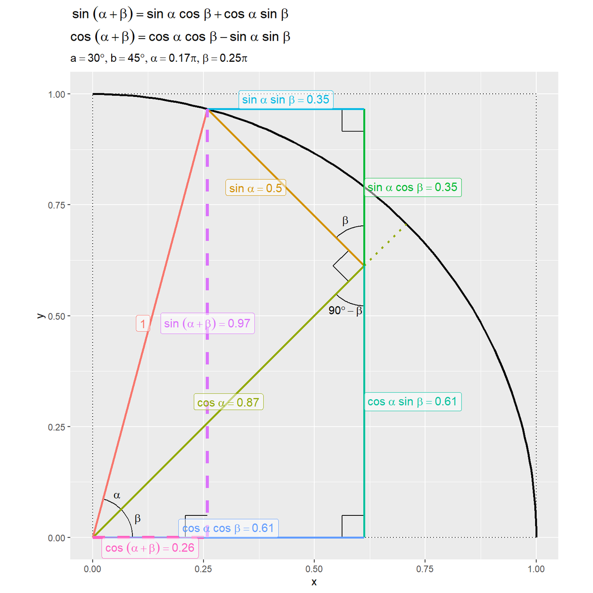
2つの破線とそれぞれ平行な実線を比較すると、次の関係が成り立つのが分かります。
アニメーションの作成
次は、角度と加法定理の関係をアニメーションで確認します。
フレームごとに変化させる角度を指定して、ラジアンに変換します。
# フレーム数を指定
frame_num <- 61

# 角度として利用する値を指定:(a,αを変化させる場合)
a_vals <- seq(from = 0, to = 60, length.out = frame_num)
b_vals <- rep(30, times = frame_num)

# 角度として利用する値を指定:(b,βを変化させる場合)
#a_vals <- rep(30, times = frame_num)
#b_vals <- seq(from = 0, to = 60, length.out = frame_num)

# ラジアンに変換
alpha_vals <- a_vals / 180 * pi
beta_vals  <- b_vals / 180 * pi
head(a_vals); head(b_vals); head(alpha_vals); head(beta_vals)
## [1] 0 1 2 3 4 5
## [1] 30 30 30 30 30 30
## [1] 0.00000000 0.01745329 0.03490659 0.05235988 0.06981317 0.08726646
## [1] 0.5235988 0.5235988 0.5235988 0.5235988 0.5235988 0.5235988
フレーム数frame_numを指定してframe_num個の角度$a, b$を作成してa_vals, b_valsとします。$a$を変化させる場合は、a_valsを一定間隔の値にして、b_valsの値を固定します。$b$を変化させる場合は、a_valsの値を固定して、b_valsを一定間隔の値にします。
作成した角度をそれぞれラジアン$\alpha, \beta$に変換してalpha_vals, beta_valsとします。
・コード(クリックで展開)
辺を描画するためのデータフレームを作成します。
# 辺の描画用
anim_segment_df <- tidyr::expand_grid(
  tibble::tibble(
    frame_i = 1:frame_num, # フレーム番号
    alpha = alpha_vals,
    beta = beta_vals
  ),
  tibble::tibble(
    fnc = c(
      "1", "sin(a)", "cos(a)", "cos(a)",
      "sin(a) cos(b)", "sin(a) cos(b)", "cos(a) sin(b)", "cos(a) sin(b)",
      "sin(a) sin(b)", "cos(a) cos(b)",
      "sin(a+b)", "cos(a+b)"
    ) |>
        factor(levels = fnc_level), # 因子レベルを設定
    type = c(
      "main", "main", "main", "sub",
      "main", "sub", "main", "sub",
      "main", "main",
      "target", "target"
    )
  )
) |> # フレームごとに受け皿(行)を複製
  dplyr::group_by(frame_i) |>
  dplyr::mutate(
    # 座標を計算
    x_from = c(
      0, cos(unique(alpha))*cos(unique(beta)), 0, cos(unique(alpha))*cos(unique(beta)),
      cos(unique(alpha))*cos(unique(beta)), cos(unique(alpha))*cos(unique(beta)), cos(unique(alpha))*cos(unique(beta)), cos(unique(alpha))*cos(unique(beta)),
      cos(unique(alpha)+unique(beta)), 0,
      cos(unique(alpha)+unique(beta)), 0
    ),
    y_from = c(
      0, cos(unique(alpha))*sin(unique(beta)), 0, cos(unique(alpha))*sin(unique(beta)),
      cos(unique(alpha))*sin(unique(beta)), sin(unique(alpha)+unique(beta)), 0, 0,
      sin(unique(alpha)+unique(beta)), 0,
      0, 0
    ),
    x_to = c(
      cos(unique(alpha)+unique(beta)), cos(unique(alpha)+unique(beta)), cos(unique(alpha))*cos(unique(beta)), cos(unique(beta)),
      cos(unique(alpha))*cos(unique(beta)), cos(unique(alpha))*cos(unique(beta)), cos(unique(alpha))*cos(unique(beta)), cos(unique(alpha))*cos(unique(beta)),
      cos(unique(alpha))*cos(unique(beta)), cos(unique(alpha))*cos(unique(beta)),
      cos(unique(alpha)+unique(beta)), cos(unique(alpha)+unique(beta))
    ),
    y_to = c(
      sin(unique(alpha)+unique(beta)), sin(unique(alpha)+unique(beta)), cos(unique(alpha))*sin(unique(beta)), sin(unique(beta)),
      sin(unique(alpha)+unique(beta)), 1.1, cos(unique(alpha))*sin(unique(beta)), -0.1,
      sin(unique(alpha)+unique(beta)), 0,
      sin(unique(alpha)+unique(beta)), 0
    ),
    # 変数ラベルを作成
    frame_label = paste0(
      "a=", a_vals[unique(frame_i)], "°, b=", b_vals[unique(frame_i)], "°",
      ", α=", round(a_vals[unique(frame_i)]/180, 2), "π, β=", round(b_vals[unique(frame_i)]/180, 2), "π"
    ) |>
      factor(
        levels = paste0(
          "a=", a_vals, "°, b=", b_vals, "°",
          ", α=", round(a_vals/180, 2), "π, β=", round(b_vals/180, 2), "π"
        )
      ) # フレーム順序を設定
  ) |>
  dplyr::ungroup() |>
  dplyr::arrange(frame_i, fnc) # 並びを統一
anim_segment_df
## # A tibble: 732 × 10
##    frame_i alpha  beta fnc           type  x_from y_from  x_to  y_to frame_label
##      <int> <dbl> <dbl> <fct>         <chr>  <dbl>  <dbl> <dbl> <dbl> <fct>
##  1       1     0 0.524 1             main   0        0   0.866   0.5 a=0°, b=3…
##  2       1     0 0.524 sin(a)        main   0.866    0.5 0.866   0.5 a=0°, b=3…
##  3       1     0 0.524 cos(a)        main   0        0   0.866   0.5 a=0°, b=3…
##  4       1     0 0.524 cos(a)        sub    0.866    0.5 0.866   0.5 a=0°, b=3…
##  5       1     0 0.524 sin(a) cos(b) main   0.866    0.5 0.866   0.5 a=0°, b=3…
##  6       1     0 0.524 sin(a) cos(b) sub    0.866    0.5 0.866   1.1 a=0°, b=3…
##  7       1     0 0.524 cos(a) sin(b) main   0.866    0   0.866   0.5 a=0°, b=3…
##  8       1     0 0.524 cos(a) sin(b) sub    0.866    0   0.866  -0.1 a=0°, b=3…
##  9       1     0 0.524 sin(a) sin(b) main   0.866    0.5 0.866   0.5 a=0°, b=3…
## 10       1     0 0.524 cos(a) cos(b) main   0        0   0.866   0   a=0°, b=3…
## # … with 722 more rows
フレーム番号と対応する角度(ラジアン)を格納したデータフレームと、関数名(色分け用)と線分のタイプ(線の装飾用)を格納したデータフレームの、全ての行の組み合わせをexpand_grid()で作成することで、フレームごとにラベル(値の受け皿となる行)を複製します。
フレームごとに(frame_i列でグループ化して)、線分の始点と終点の座標を計算します。処理の仕方は異なりますが「グラフの作成」のときと同様に計算します。ただし、角度列alpha, betaは行数分の値を持つので、unique()で1つの値にして計算に使います。
また、フレーム切替用のラベル列frame_labelを作成します。因子のレベルがフレームの順番に対応します。
関数名ラベルを描画するためのデータフレームを作成します。
# 関数名ラベルの描画用
anim_segment_label_df <- anim_segment_df |>
  dplyr::filter(type %in% c("main", "target")) |> # 補助線を除去
  dplyr::group_by(frame_i, fnc) |> # 中点の計算用
  dplyr::mutate(
    # 線分の中点に配置
    x = median(c(x_from, x_to)),
    y = median(c(y_from, y_to))
  ) |>
  dplyr::select(frame_i, frame_label, fnc, alpha, beta, x, y) |>
  dplyr::group_by(frame_i) |>
  dplyr::mutate(
    # ラベルが重ならないように調整
    h = c(1.0, 1.0, 0.5, 0.0, 0.0, 0.5, 0.5, 0.5, 0.5),
    v = c(0.5, 0.5, 0.5, 0.5, 0.5, 0.0, 0.0, 0.5, 1.0),
    # ラベルを作成
    fnc_label = c(
      "1",
      paste0("sin~alpha==", round(sin(unique(alpha)), digits = 2)),
      paste0("cos~alpha==", round(cos(unique(alpha)), digits = 2)),
      paste0("sin~alpha ~ cos~beta==", round(sin(unique(alpha))*cos(unique(beta)), digits = 2)),
      paste0("cos~alpha ~ sin~beta==", round(cos(unique(alpha))*sin(unique(beta)), digits = 2)),
      paste0("sin~alpha ~ sin~beta==", round(sin(unique(alpha))*sin(unique(beta)), digits = 2)),
      paste0("cos~alpha ~ cos~beta==", round(cos(unique(alpha))*cos(unique(beta)), digits = 2)),
      paste0("sin~(alpha+beta)==", round(sin(unique(alpha)+unique(beta)), digits = 2)),
      paste0("cos~(alpha+beta)==", round(cos(unique(alpha)+unique(beta)), digits = 2))
    )
  ) |>
  dplyr::ungroup() |>
  dplyr::arrange(frame_i, fnc) # 並びを統一
anim_segment_label_df
##    frame_i frame_label    fnc      alpha  beta     x     y     h     v fnc_label
##      <int> <fct>          <fct>    <dbl> <dbl> <dbl> <dbl> <dbl> <dbl> <chr>
##  1       1 a=0°, b=30°, … 1       0      0.524 0.433 0.25    1     0.5 1
##  2       1 a=0°, b=30°, … sin(a)  0      0.524 0.866 0.5     1     0.5 sin~alph…
##  3       1 a=0°, b=30°, … cos(a)  0      0.524 0.433 0.25    0.5   0.5 cos~alph…
##  4       1 a=0°, b=30°, … sin(a)… 0      0.524 0.866 0.5     0     0.5 sin~alph…
##  5       1 a=0°, b=30°, … cos(a)… 0      0.524 0.866 0.25    0     0.5 cos~alph…
##  6       1 a=0°, b=30°, … sin(a)… 0      0.524 0.866 0.5     0.5   0   sin~alph…
##  7       1 a=0°, b=30°, … cos(a)… 0      0.524 0.433 0       0.5   0   cos~alph…
##  8       1 a=0°, b=30°, … sin(a+… 0      0.524 0.866 0.25    0.5   0.5 sin~(alp…
##  9       1 a=0°, b=30°, … cos(a+… 0      0.524 0.433 0       0.5   1   cos~(alp…
## 10       2 a=1°, b=30°, … 1       0.0175 0.524 0.429 0.258   1     0.5 1
## # … with 539 more rows
補助線を取り除いて、フレームと辺ごとに(frame_i, fnc列でグループ化して)、「グラフの作成」のときと同様に処理します。
直角を示すためのデータフレームを作成します。
# 直角マークの描画用
d <- 0.05
anim_right_angle_df <- tidyr::expand_grid(
  tibble::tibble(
    frame_i = 1:frame_num, # フレーム番号
    alpha = alpha_vals,
    beta = beta_vals
  ),
  group = rep(1:4, each = 3) # 角ラベル
) |>
  dplyr::group_by(frame_i) |> # 値の作成用
  dplyr::mutate(
    x = c(
      cos(unique(alpha)+unique(beta)), cos(unique(alpha)+unique(beta))-d, cos(unique(alpha)+unique(beta))-d,
      cos(unique(alpha))*cos(unique(beta)), cos(unique(alpha))*cos(unique(beta))-d, cos(unique(alpha))*cos(unique(beta))-d,
      cos(unique(alpha))*cos(unique(beta))-d, cos(unique(alpha))*cos(unique(beta))-d, cos(unique(alpha))*cos(unique(beta)),
      cos(unique(alpha))*cos(unique(beta)) + c(cos(unique(beta)+0.5*pi)*d, cos(unique(beta)+0.5*pi)*d+cos(unique(beta)+pi)*d, cos(unique(beta)+pi)*d)
    ),
    y = c(
      d, d, 0,
      d, d, 0,
      sin(unique(alpha)+unique(beta)), sin(unique(alpha)+unique(beta))-d, sin(unique(alpha)+unique(beta))-d,
      cos(unique(alpha))*sin(unique(beta)) + c(sin(unique(beta)+0.5*pi)*d, sin(unique(beta)+0.5*pi)*d+sin(unique(beta)+pi)*d, sin(unique(beta)+pi)*d)
    ),
    # 変数ラベルを作成
    frame_label = paste0(
      "a=", a_vals[unique(frame_i)], "°, b=", b_vals[unique(frame_i)], "°",
      ", α=", round(a_vals[unique(frame_i)]/180, 2), "π, β=", round(b_vals[unique(frame_i)]/180, 2), "π"
    ) |>
      factor(
        levels = paste0(
          "a=", a_vals, "°, b=", b_vals, "°",
          ", α=", round(a_vals/180, 2), "π, β=", round(b_vals/180, 2), "π"
        )
      ) # フレーム順序を設定
  ) |>
  dplyr::ungroup()
anim_right_angle_df
## # A tibble: 732 × 7
##    frame_i alpha  beta group     x     y frame_label
##      <int> <dbl> <dbl> <int> <dbl> <dbl> <fct>
##  1       1     0 0.524     1 0.866 0.05  a=0°, b=30°, α=0π, β=0.17π
##  2       1     0 0.524     1 0.816 0.05  a=0°, b=30°, α=0π, β=0.17π
##  3       1     0 0.524     1 0.816 0     a=0°, b=30°, α=0π, β=0.17π
##  4       1     0 0.524     2 0.866 0.05  a=0°, b=30°, α=0π, β=0.17π
##  5       1     0 0.524     2 0.816 0.05  a=0°, b=30°, α=0π, β=0.17π
##  6       1     0 0.524     2 0.816 0     a=0°, b=30°, α=0π, β=0.17π
##  7       1     0 0.524     3 0.816 0.5   a=0°, b=30°, α=0π, β=0.17π
##  8       1     0 0.524     3 0.816 0.45  a=0°, b=30°, α=0π, β=0.17π
##  9       1     0 0.524     3 0.866 0.45  a=0°, b=30°, α=0π, β=0.17π
## 10       1     0 0.524     4 0.841 0.543 a=0°, b=30°, α=0π, β=0.17π
## # … with 722 more rows
フレームごとに角度に応じて、直角マークの頂点の座標を計算します。
先に作成したフレーム切り替え用のラベル列と一致するようにラベルを作成します。
鋭角を示すためのデータフレームを作成します。
# 角度マーク(扇形)の描画用
d <- 0.09
anim_angle_df <- tibble::tibble(
  frame_i = 1:frame_num, # フレーム番号
  a = a_vals,
  b = b_vals,
  alpha = alpha_vals,
  beta = beta_vals
) |>
  dplyr::group_by(frame_i, a, b, alpha, beta) |> # 値の作成用
  dplyr::summarise(
    # 原点を中心としたときの角度
    c = c(
      seq(from = 0, to = b, by = 1),
      seq(from = b, to = a+b, by = 1),
      seq(from = 90, to = 90+b, by = 1),
      seq(from = 180+b, to = 270, by = 1)
    ),
    .groups = "drop"
  ) |>
  dplyr::group_by(frame_i) |>
  dplyr::mutate(
    # 原点を中心としたときの角度
    theta = c / 180 * pi,
    group = c(
      rep("b1", times = length(seq(from = 0, to = unique(b), by = 1))),
      rep("a", times = length(seq(from = unique(b), to = unique(a)+unique(b), by = 1))),
      rep("b2", times = length(seq(from = 90, to = 90+unique(b), by = 1))),
      rep("90-b", times = length(seq(from = 180+unique(b), to = 270, by = 1)))
    ) |> # 角ラベル
      factor(levels = c("b1", "a", "b2", "90-b")), # 因子レベルを設定
    # 原点を中心としたときの座標
    x = cos(theta) * d,
    y = sin(theta) * d,
    # 角ごとに配置
    x = x + c(
      rep(0, times = length(seq(from = 0, to = unique(b), by = 1))),
      rep(0, times = length(seq(from = unique(b), to = unique(a)+unique(b), by = 1))),
      rep(cos(unique(alpha))*cos(unique(beta)), times = length(seq(from = 90, to = 90+unique(b), by = 1))),
      rep(cos(unique(alpha))*cos(unique(beta)), times = length(seq(from = 180+unique(b), to = 270, by = 1)))
    ),
    y = y + c(
      rep(0, times = length(seq(from = 0, to = unique(b), by = 1))),
      rep(0, times = length(seq(from = unique(b), to = unique(a)+unique(b), by = 1))),
      rep(cos(unique(alpha))*sin(unique(beta)), times = length(seq(from = 90, to = 90+unique(b), by = 1))),
      rep(cos(unique(alpha))*sin(unique(beta)), times = length(seq(from = 180+unique(b), to = 270, by = 1)))
    ),
    # 変数ラベルを作成
    frame_label = paste0(
      "a=", unique(a), "°, b=", unique(b), "°",
      ", α=", round(a_vals[unique(frame_i)]/180, 2), "π, β=", round(b_vals[unique(frame_i)]/180, 2), "π"
    ) |>
      factor(
        levels = paste0(
          "a=", a_vals, "°, b=", b_vals, "°",
          ", α=", round(a_vals/180, 2), "π, β=", round(b_vals/180, 2), "π"
        )
      ) # フレーム順序を設定
  ) |>
  dplyr::ungroup() |>
  dplyr::arrange(frame_i, group) # 並びを統一
anim_angle_df
## # A tibble: 9,394 × 11
##    frame_i     a     b alpha  beta     c  theta group      x       y frame_label
##      <int> <dbl> <dbl> <dbl> <dbl> <dbl>  <dbl> <fct>  <dbl>   <dbl> <fct>
##  1       1     0    30     0 0.524     0 0      b1    0.09   0       a=0°, b=3…
##  2       1     0    30     0 0.524     1 0.0175 b1    0.0900 0.00157 a=0°, b=3…
##  3       1     0    30     0 0.524     2 0.0349 b1    0.0899 0.00314 a=0°, b=3…
##  4       1     0    30     0 0.524     3 0.0524 b1    0.0899 0.00471 a=0°, b=3…
##  5       1     0    30     0 0.524     4 0.0698 b1    0.0898 0.00628 a=0°, b=3…
##  6       1     0    30     0 0.524     5 0.0873 b1    0.0897 0.00784 a=0°, b=3…
##  7       1     0    30     0 0.524     6 0.105  b1    0.0895 0.00941 a=0°, b=3…
##  8       1     0    30     0 0.524     7 0.122  b1    0.0893 0.0110  a=0°, b=3…
##  9       1     0    30     0 0.524     8 0.140  b1    0.0891 0.0125  a=0°, b=3…
## 10       1     0    30     0 0.524     9 0.157  b1    0.0889 0.0141  a=0°, b=3…
## # … with 9,384 more rows
フレームごとに角度に応じて、角度マークを描画するための点の角度をsummarise()で作成して、それぞれ座標を計算します。
角度ラベルを描画するためのデータフレームを作成します。
# 角度ラベルの描画用
d <- 0.11
anim_angle_label_df <- anim_angle_df |>
  dplyr::group_by(frame_i, frame_label, alpha, beta, group) |> # 中点の計算用
  dplyr::summarise(
    # 角度の中点に配置
    c = median(c), .groups = "drop"
  ) |>
  dplyr::mutate(
    # 原点を中心としたときの座標
    theta = c / 180 * pi,
    x = cos(theta) * d,
    y = sin(theta) * d
  ) |>
  dplyr::group_by(frame_i) |>
  dplyr::mutate(
    # 角ごとに配置
    x = x + c(0, 0, cos(unique(alpha))*cos(unique(beta)), cos(unique(alpha))*cos(unique(beta))),
    y = y + c(0, 0, cos(unique(alpha))*sin(unique(beta)), cos(unique(alpha))*sin(unique(beta))),
    label = c("beta", "alpha", "beta", "90*degree-beta") # 角ラベル
  ) |>
  dplyr::ungroup()
anim_angle_label_df
## # A tibble: 244 × 10
##    frame_i frame_label      alpha  beta group     c theta      x      y label
##      <int> <fct>            <dbl> <dbl> <fct> <dbl> <dbl>  <dbl>  <dbl> <chr>
##  1       1 a=0°, b=30°, α… 0      0.524 b1     15   0.262 0.106  0.0285 beta
##  2       1 a=0°, b=30°, α… 0      0.524 a      30   0.524 0.0953 0.055  alpha
##  3       1 a=0°, b=30°, α… 0      0.524 b2    105   1.83  0.838  0.606  beta
##  4       1 a=0°, b=30°, α… 0      0.524 90-b  240   4.19  0.811  0.405  90*degr…
##  5       2 a=1°, b=30°, α… 0.0175 0.524 b1     15   0.262 0.106  0.0285 beta
##  6       2 a=1°, b=30°, α… 0.0175 0.524 a      30.5 0.532 0.0948 0.0558 alpha
##  7       2 a=1°, b=30°, α… 0.0175 0.524 b2    105   1.83  0.837  0.606  beta
##  8       2 a=1°, b=30°, α… 0.0175 0.524 90-b  240   4.19  0.811  0.405  90*degr…
##  9       3 a=2°, b=30°, α… 0.0349 0.524 b1     15   0.262 0.106  0.0285 beta
## 10       3 a=2°, b=30°, α… 0.0349 0.524 a      31   0.541 0.0943 0.0567 alpha
## # … with 234 more rows
フレームと角ごとに(frame_i, group列と中央値の計算後に利用する列でグループ化して)、summaraise()で角度の中点を計算して、それぞれ座標を計算します。
加法定理の可視化アニメーションを作成します。
# 加法定理の可視化アニメーションの作図
anim <- ggplot() +
  geom_path(data = sector_df,
            mapping = aes(x = x, y = y),
            size = 1) + # 単位円
  geom_path(data = square_df,
            mapping = aes(x = x, y = y),
            linetype = "dotted") + # 単位正方形
  geom_path(data = anim_right_angle_df,
            mapping = aes(x = x, y = y, group = group)) + # 直角マーク
  geom_path(data = anim_angle_df,
            mapping = aes(x = x, y = y, group = group)) + # 角度マーク
  geom_text(data = anim_angle_label_df,
            mapping = aes(x = x, y = y, label = label), parse = TRUE) + # 角度ラベル
  geom_segment(data = anim_segment_df,
               mapping = aes(x = x_from, y = y_from, xend = x_to, yend = y_to,
                             color = fnc, size = type, linetype = type)) + # 関数の線分
  geom_label(data = anim_segment_label_df,
             mapping = aes(x = x, y = y, label = fnc_label, color = fnc, hjust = h, vjust = v),
             parse = TRUE, alpha = 0.5, size = 4) + # 関数ラベル
  gganimate::transition_manual(frame = frame_label) +
  scale_size_manual(breaks = c("main", "sub", "target"),
                    values = c(1, 1, 1.5)) + #  目的の線を強調
  scale_linetype_manual(breaks = c("main", "sub", "target"),
                        values = c("solid", "dotted", "dashed")) + #  目的の線を強調
  theme(legend.position = "none") + # 凡例を非表示
  coord_fixed(ratio = 1, clip = "off", xlim = c(0, 1), ylim = c(0, 1)) + # アスペクト比
  labs(title = parse(text = title_label),
       subtitle = "{current_frame}")

# gif画像を作成
gganimate::animate(plot = anim, nframe = frame_num, fps = 10, width = 600, height = 600)
transition_manual()にフレームの順序を表す列を指定します。この例では、因子型のラベルのレベルの順に描画されます。
animate()のnframes引数にフレーム数、fps引数に1秒当たりのフレーム数を指定します。fps引数の値が大きいほどフレームが早く切り替わります。ただし、値が大きいと意図通りに動作しません。

$\alpha + \beta$が$0^{\circ}$から$90^{\circ}$に近付くほど、$\sin(\alpha + \beta)$が0から1に、$\cos(\alpha + \beta)$が1から0に近付くのを確認できます。
この記事では、2角の和について可視化しました。次の記事では、2角の差について可視化します。
参考書籍
- 『三角関数(改定第3版)』(Newton別冊)ニュートンプレス,2022年.
おわりに
とりあえず本の図を再現したくなる今日この頃です。この図だと2つの式しか説明できないことに途中で気付きました。他の式の図もあるもんだと思って調べてみたら、あんまりないんですね。2つだけ書いてもなぁでもお蔵入りもなぁと悩んだ結果、自分で図を考えてみました。それが上手くいく予定なので、こっちをアップしました。
数式での導出もしてみたいのですが、それはまたの機会に。
【次の内容】