はじめに
『Rが生産性を高める 〜データ分析ワークフロー効率化の実践』(R登山本)の内容を実際にやってみた記録や気になったことのメモです。
この記事は、6章を読んでやってみた内容です。本とあわせて読んでください。
【前の内容】
【この記事の内容】
バーチャートレースによる頻出語の可視化
前回は、指定した月に登場した単語の頻度を棒グラフで可視化しました。今回は、期間を指定して、月ごとの単語の推移をバーチャートレースで可視化します。
次のパッケージを利用します。
# 利用するパッケージ
library(RMeCab)
library(tidyverse)
library(gganimate)
RMeCabは、RからMeCabを利用するためのパッケージです。形態素解析器MeCabがインストールされている必要があります。
gganimateは、ggplot2を使ったグラフのアニメーション(gif画像)を作成するためのパッケージです。
この記事では、基本的にパッケージ名::関数名()の記法を使うので、パッケージを読み込む必要はありません。
ただし、パイプ演算子%>%を使うためmagrittrと、作図コードがごちゃごちゃしないようにパッケージ名を省略するためggplot2は読み込む必要があります。
形態素解析
まずは、形態素解析を行い、文章を単語(形態素)に分解します。利用するテキストについては「Chapter 6:ブログの内容を棒グラフで可視化してみた【R登山本】 - からっぽのしょこ」を参照してください。
フォルダを指定して、フォルダ内の全てのテキストに対して形態素解析を行います。
# フォルダパスを指定
dir_path <- "フォルダ名"

# MeCabによる形態素解析
mecab_df <- RMeCab::docDF(target = dir_path, type = 1) %>%
  tibble::as_tibble()
head(mecab_df)
## # A tibble: 6 x 41
##   TERM   POS1  POS2     `2018_12.txt` `2019_01.txt` `2019_02.txt` `2019_03.txt`
##   <chr>  <chr> <chr>            <int>         <int>         <int>         <int>
## 1 "!"    名詞  サ変接続             2             1             0             0
## 2 "!!"   名詞  サ変接続             0             1             0             0
## 3 "!\""  名詞  サ変接続             0             0             0             0
## 4 "!\")" 名詞  サ変接続             0             0             0             0
## 5 "!$"   名詞  サ変接続             0             0             0             0
## 6 "!="   名詞  サ変接続             0             0             0             1
## # ... with 34 more variables: `2019_04.txt` <int>, `2019_05.txt` <int>,
## #   `2019_06.txt` <int>, `2019_07.txt` <int>, `2019_08.txt` <int>,
## #   `2019_09.txt` <int>, `2019_12.txt` <int>, `2020_01.txt` <int>,
## #   `2020_02.txt` <int>, `2020_04.txt` <int>, `2020_05.txt` <int>,
## #   `2020_06.txt` <int>, `2020_07.txt` <int>, `2020_08.txt` <int>,
## #   `2020_09.txt` <int>, `2020_10.txt` <int>, `2020_11.txt` <int>,
## #   `2020_12.txt` <int>, `2021_01.txt` <int>, `2021_02.txt` <int>, ...
RMeCabパッケージのdocDF()で、形態素解析を行います。target(第1引数)にフォルダパス、type引数に1を指定します。
TERM列は単語(形態素)、POS1列は品詞大分類、POS2列は品詞小分類です。4列目以降は各テキストに対応していて、ファイル名が列名になり、そのテキストにおける単語の頻度が値になります。
以上で、文章を単語に分かち書きできました。
単語の集計
次に、記事の内容を反映する単語を抽出します。
記号類や意味を持たない単語などを取り除く設定をします。
# 単語数を指定
max_rank <- 100

# 利用する品詞を指定
pos1_vec <- c("名詞", "動詞", "形容詞")
pos2_vec <- c("一般", "固有名詞", "サ変接続", "形容動詞語幹", "ナイ形容詞語幹", "自立")

# 削除する単語を指定
stopword_symbol_vec <- c("\\(", "\\)", "\\{", "\\}", "\\[", "]", "「", "」", ",", "_", "--", "!", "#", "\\.", "\\$", "\\\\")
stopword_term_vec <- c("る", "ある", "する", "せる", "できる", "なる", "やる", "れる", "いい", "ない")
利用する品詞大分類をpos1_vec、品詞小分類をpos2_vecとして指定します。
削除する記号と単語をstopword_***_vecに指定します。正規表現に使われる記号の場合は、エスケープ文字\\を付ける必要があります。
それぞれ結果を見ながら指定してください。
利用する単語を抽出して、出現頻度を再集計し、出現頻度の上位単語を抽出します。
# 頻出語を抽出
rank_df <- mecab_df %>%
  dplyr::filter(POS1 %in% pos1_vec) %>% # 指定した品詞大分類を抽出
  dplyr::filter(POS2 %in% pos2_vec) %>% # 指定した品詞小分類を抽出
  dplyr::filter(!stringr::str_detect(TERM, pattern = paste0(stopword_symbol_vec, collapse = "|"))) %>% # 不要な記号を削除
  dplyr::filter(!stringr::str_detect(TERM, pattern = paste0(stopword_term_vec, collapse = "|"))) %>% # 不要な単語を削除
  dplyr::select(term = TERM, !c("POS1", "POS2")) %>% # 単語と頻度の列を取り出し
  tidyr::pivot_longer(cols = !term, names_to = "date", values_to = "frequency") %>% # 頻度列をまとめる
  dplyr::mutate(
    date = date %>%
      stringr::str_remove(pattern = ".txt") %>%
      stringr::str_replace(pattern = "_", replacement = "-") %>%
      stringr::str_c("-01") %>%
      lubridate::as_date()
  ) %>% # 日付情報に変換
  dplyr::group_by(term, date) %>% # 単語と月でグループ化
  dplyr::summarise(frequency = sum(frequency), .groups = "drop") %>% # 頻度を合計
  dplyr::arrange(date, frequency) %>% # 昇順に並び替え
  dplyr::group_by(date) %>% # 月でグループ化
  dplyr::mutate(ranking = dplyr::row_number(-frequency)) %>% # 月ごとにランク付け
  dplyr::ungroup() %>% # グループ化を解除
  dplyr::filter(ranking <= max_rank) %>% # 頻度上位単語を抽出
  dplyr::arrange(date, ranking) # 昇順に並び替え
head(rank_df)
## # A tibble: 6 x 4
##   term   date       frequency ranking
##   <chr>  <date>         <int>   <int>
## 1 "\""   2018-12-01       264       1
## 2 "<-"   2018-12-01       161       2
## 3 "="    2018-12-01       138       3
## 4 "単語" 2018-12-01        79       4
## 5 "tmp"  2018-12-01        64       5
## 6 "%>%"  2018-12-01        60       6
filter()で単語を抽出して、pivot_longer()で頻度列をまとめて、summarise()で重複語の頻度を合計して、arrange()とhead()で頻度が多い単語を抽出します。
処理の塊ごとに確認していきます。
・処理の確認(クリックで展開)
利用する品詞を抽出して、不要な単語を削除します。
# 頻出語を抽出
tmp1_df <- mecab_df %>%
  dplyr::filter(POS1 %in% pos1_vec) %>% # 指定した品詞大分類を抽出
  dplyr::filter(POS2 %in% pos2_vec) %>% # 指定した品詞小分類を抽出
  dplyr::filter(!stringr::str_detect(TERM, pattern = paste0(stopword_symbol_vec, collapse = "|"))) %>% # 不要な記号を削除
  dplyr::filter(!stringr::str_detect(TERM, pattern = paste0(stopword_term_vec, collapse = "|"))) %>% # 不要な単語を削除
  dplyr::select(term = TERM, !c("POS1", "POS2")) # 単語と頻度の列を取り出し
tmp1_df
## # A tibble: 8,370 x 39
##    term    `2018_12.txt` `2019_01.txt` `2019_02.txt` `2019_03.txt` `2019_04.txt`
##    <chr>           <int>         <int>         <int>         <int>         <int>
##  1 "\""              264          3567             6           263            78
##  2 "\"\""              5             0             0             0             0
##  3 "\"%"               0             0             0            10             2
##  4 "\"&\""             0             0             0             0             0
##  5 "\"'\""             0             1             0             0             0
##  6 "\"*\""            28             0             0             0             0
##  7 "\"-"               0             0             0             0             0
##  8 "\":\""             0             0             0             0             0
##  9 "\"<"               0             0             0             0             0
## 10 "\"===~             0             0             0             0             0
## # ... with 8,360 more rows, and 33 more variables: `2019_05.txt` <int>,
## #   `2019_06.txt` <int>, `2019_07.txt` <int>, `2019_08.txt` <int>,
## #   `2019_09.txt` <int>, `2019_12.txt` <int>, `2020_01.txt` <int>,
## #   `2020_02.txt` <int>, `2020_04.txt` <int>, `2020_05.txt` <int>,
## #   `2020_06.txt` <int>, `2020_07.txt` <int>, `2020_08.txt` <int>,
## #   `2020_09.txt` <int>, `2020_10.txt` <int>, `2020_11.txt` <int>,
## #   `2020_12.txt` <int>, `2021_01.txt` <int>, `2021_02.txt` <int>, ...
filter()で利用する単語を抽出します。この処理については前回の記事を参照してください。
select()で、単語列と頻度列を取り出して、扱いやすいように列名を変更します。
全てのテキストの頻度列をまとめます。
tmp2_df <- tmp1_df %>%
  tidyr::pivot_longer(cols = !term, names_to = "date", values_to = "frequency") %>% # 頻度列をまとめる
  dplyr::mutate(
    date = date %>%
      stringr::str_remove(pattern = ".txt") %>%
      stringr::str_replace(pattern = "_", replacement = "-") %>%
      stringr::str_c("-01") %>%
      lubridate::as_date()
  ) # 日付情報に変換
tmp2_df
## # A tibble: 318,060 x 3
##    term  date       frequency
##    <chr> <date>         <int>
##  1 "\""  2018-12-01       264
##  2 "\""  2019-01-01      3567
##  3 "\""  2019-02-01         6
##  4 "\""  2019-03-01       263
##  5 "\""  2019-04-01        78
##  6 "\""  2019-05-01        53
##  7 "\""  2019-06-01        94
##  8 "\""  2019-07-01        58
##  9 "\""  2019-08-01        49
## 10 "\""  2019-09-01       142
## # ... with 318,050 more rows
pivot_longer()で、各テキストの頻度列を、ファイル名列(date)と頻度列(frequency)にまとめます。
ファイル名列を日付列に変換します。ファイル名はyyyy_mm.txtなので、削除str_remove()・置換str_replace()・結合str_c()を使ってyyyy-mm-01にして、さらにas_date()でDate型に変換します。
頻度を再集計します。
tmp3_df <- tmp2_df %>%
  dplyr::group_by(term, date) %>% # 単語と月でグループ化
  dplyr::summarise(frequency = sum(frequency), .groups = "drop") %>% # 頻度を合計
  dplyr::arrange(date, frequency) # 昇順に並び替え
tmp3_df
## # A tibble: 263,454 x 3
##    term  date       frequency
##    <chr> <date>         <int>
##  1 ''    2018-12-01         0
##  2 ''='  2018-12-01         0
##  3 '-    2018-12-01         0
##  4 '-':  2018-12-01         0
##  5 '!'  2018-12-01         0
##  6 '&    2018-12-01         0
##  7 '*'   2018-12-01         0
##  8 '**'  2018-12-01         0
##  9 '***' 2018-12-01         0
## 10 '、   2018-12-01         0
## # ... with 263,444 more rows
品詞の情報を落としたので、品詞の異なる同一単語が重複して存在することになります。
そこで、group_by()で単語と月(テキスト)でグループ化して、summarise()とsum()で頻度を合算します。
頻度が多い順にランキングを付けます。
tmp4_df <- tmp3_df %>% # 昇順に並び替え
  dplyr::group_by(date) %>% # 月でグループ化
  dplyr::mutate(ranking = dplyr::row_number(-frequency)) %>% # 月ごとにランク付け
  dplyr::ungroup() %>% # グループ化を解除
  dplyr::filter(ranking <= max_rank) %>% # 頻度上位単語を抽出
  dplyr::arrange(date, ranking) # 昇順に並び替え
tmp4_df
## # A tibble: 3,800 x 4
##    term       date       frequency ranking
##    <chr>      <date>         <int>   <int>
##  1 "\""       2018-12-01       264       1
##  2 "<-"       2018-12-01       161       2
##  3 "="        2018-12-01       138       3
##  4 "単語"     2018-12-01        79       4
##  5 "tmp"      2018-12-01        64       5
##  6 "%>%"      2018-12-01        60       6
##  7 "名詞"     2018-12-01        53       7
##  8 "file"     2018-12-01        48       8
##  9 "data"     2018-12-01        47       9
## 10 "テキスト" 2018-12-01        45      10
## # ... with 3,790 more rows
月でグループ化することで、テキストごとに処理できます。
row_number()で通し番号を付けます。
指定した単語数までの上位単語を抽出します。
以上で、前処理ができました。
バーチャートレースの作成
最後に、単語の出現頻度の推移をバーチャートレースで可視化します。
フレーム数を指定します。
# フレーム数を取得
n <- length(unique(rank_df[["date"]]))

# 遷移フレーム数を指定
t <- 8

# 停止フレーム数を指定
s <- 2
基本となるフレーム数(月の数)をnとします。
現月と次月のグラフを繋ぐアニメーションのフレーム数をtとして、整数を指定します。
各月のグラフで一時停止するフレーム数をsとして、整数を指定します。
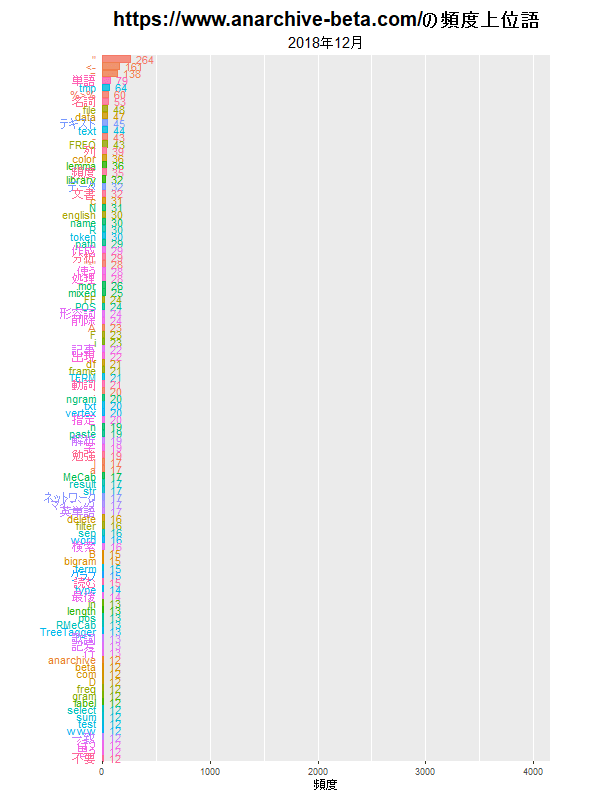
出現頻度のバーチャートレースを作成します。1つ目は、y軸を最大値で固定して描画します。
# バーチャートレースを作成:(y軸固定)
anim <- ggplot(rank_df, aes(x = ranking, y = frequency, fill = term, color = term)) +
  geom_bar(stat = "identity", width = 0.9, alpha = 0.8) + # 棒グラフ
  geom_text(aes(y = 0, label = paste(term, " ")), hjust = 1) + # 単語ラベル
  geom_text(aes(label = paste(" ", frequency)), hjust = 0) + # 頻度ラベル
  gganimate::transition_states(states = date, transition_length = t, state_length = s, wrap = FALSE) + # フレーム
  gganimate::ease_aes("cubic-in-out") + # アニメーションの緩急
  coord_flip(clip = "off", expand = FALSE) + # 軸の入替
  scale_x_reverse() + # x軸の反転
  theme(
    axis.title.y = element_blank(), # 縦軸のラベル
    axis.text.y = element_blank(), # 縦軸の目盛ラベル
    axis.ticks.y = element_blank(), # 縦軸の目盛指示線
    #panel.grid.major.x = element_line(color = "grey", size = 0.1), # 横軸の主目盛線
    panel.grid.major.y = element_blank(), # 縦軸の主目盛線
    panel.grid.minor.y = element_blank(), # 縦軸の補助目盛線
    panel.border = element_blank(), # グラフ領域の枠線
    #panel.background = element_blank(), # グラフ領域の背景
    plot.title = element_text(color = "black", face = "bold", size = 20, hjust = 0.5), # 全体のタイトル
    plot.subtitle = element_text(color = "black", size = 15, hjust = 0.5), # 全体のサブタイトル
    plot.margin = margin(t = 10, r = 50, b = 10, l = 100, unit = "pt"), # 全体の余白
    legend.position = "none" # 凡例の表示位置
  ) + # 図の体裁
  labs(
    title = "https://www.anarchive-beta.com/の頻度上位語",
    subtitle = "{lubridate::year(closest_state)}年{lubridate::month(closest_state)}月",
    y = "頻度"
  ) # ラベル
2つ目は、グラフごとにy軸の範囲が変化します。
# バーチャートレースを作成:(y軸可変)
anim <- ggplot(rank_df, aes(x = ranking, y = frequency, fill = term, color = term)) +
  geom_bar(stat = "identity", width = 0.9, alpha = 0.8) + # 棒グラフ
  geom_text(aes(y = 0, label = paste(term, " ")), hjust = 1) + # 単語ラベル
  geom_text(aes(label = paste(" ", frequency, "回")), hjust = 0) + # 頻度ラベル
  gganimate::transition_states(states = date, transition_length = t, state_length = s, wrap = FALSE) + # フレーム
  gganimate::ease_aes("cubic-in-out") + # アニメーションの緩急
  coord_flip(clip = "off", expand = FALSE) + # 軸の入替
  scale_x_reverse() + # x軸の反転
  gganimate::view_follow(fixed_x = TRUE) + # フレームごとに表示範囲を調整
  theme(
    axis.title.x = element_blank(), # 横軸のラベル
    axis.title.y = element_blank(), # 縦軸のラベル
    axis.text.x = element_blank(), # 横軸の目盛ラベル
    axis.text.y = element_blank(), # 縦軸の目盛ラベル
    axis.ticks.x = element_blank(), # 横軸の目盛指示線
    axis.ticks.y = element_blank(), # 縦軸の目盛指示線
    #panel.grid.major.x = element_line(color = "grey", size = 0.1), # 横軸の主目盛線
    panel.grid.major.y = element_blank(), # 縦軸の主目盛線
    panel.grid.minor.x = element_blank(), # 横軸の補助目盛線
    panel.grid.minor.y = element_blank(), # 縦軸の補助目盛線
    panel.border = element_blank(), # グラフ領域の枠線
    #panel.background = element_blank(), # グラフ領域の背景
    plot.title = element_text(color = "black", face = "bold", size = 20, hjust = 0.5), # 全体のタイトル
    plot.subtitle = element_text(color = "black", size = 15, hjust = 0.5), # 全体のサブタイトル
    plot.margin = margin(t = 10, r = 50, b = 10, l = 100, unit = "pt"), # 全体の余白
    legend.position = "none" # 凡例の表示位置
  ) + # 図の体裁
  labs(
    title = "https://www.anarchive-beta.com/の頻度上位語",
    subtitle = "{lubridate::year(closest_state)}年{lubridate::month(closest_state)}月"
  ) # ラベル
バーチャートレースの作成については「【R】バーチャートレースのアニメーションの作図【gganimate】 - からっぽのしょこ」を参照してください。
animate()でgif画像を作成します。
# gif画像を作成
g <- gganimate::animate(
  plot = anim, nframes = n*(t+s), fps = t+s, width = 900, height = 1200
)
g
plot引数にグラフ、nframes引数にフレーム数、fps引数に1秒当たりのフレーム数を指定します。
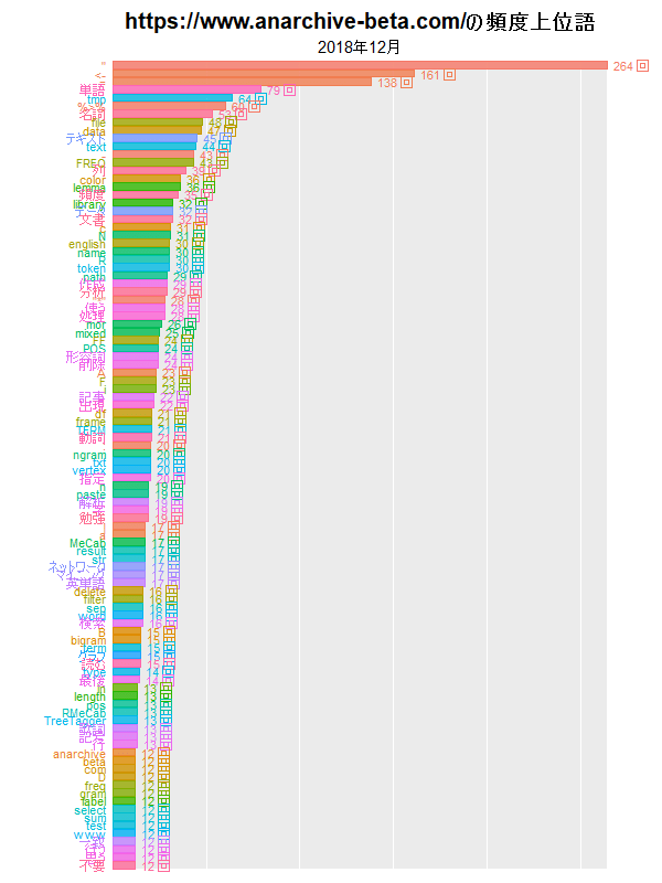
y軸(横軸)を可変にすると、月ごとに正規化されたようなグラフになり、単語の総数(記事の数)の影響が緩和されます。
(ブログの問題で小さいサイズにしました。もう少し大きいのを下に貼っています。)
anim_save()でgif画像を保存します。
# gif画像を保存
gganimate::anim_save(filename = "BarChartRace.gif", animation = g)
filename引数にファイルパス("(保存する)フォルダ名/(作成する)ファイル名.gif")、animation引数に作成したgif画像を指定します。
動画を作成する場合は、renderer引数を指定します。
# 動画を作成と保存
m <- gganimate::animate(
  plot = anim, nframes = n*(t+s), fps = t+s, width = 900, height = 1200,
  renderer = gganimate::av_renderer(file = "BarChartRace.mp4")
)
renderer引数に、レンダリング方法に応じた関数を指定します。この例では、av_renderer()を使います。
av_renderer()のfile引数に保存先のファイルパス("(保存する)フォルダ名/(作成する)ファイル名.mp4")を指定します。
もう少し大きいサイズをここに貼っておきました。
ブログに登場する単語の変化 pic.twitter.com/tO1JS79N68
— しょこ📚 (@anemptyarchive) April 26, 2022
以上で、ブログ記事の変化を可視化できました。
参考書籍
- 「Rが生産性を高める 〜データ分析ワークフロー効率化の実践」igjit・atusy・hanaori 著,技術評論社,2022年.
おわりに
時期によって扱う内容が変わり登場する単語も変わる?トピックモデルをしないと!
【次の内容】
つづく