はじめに

　R言語のgganimateパッケージを使ってグラフを動かそうシリーズです。
　この記事では、1次元のランダムウォークのアニメーションを作成します。

【他の内容】

【目次】

はじめに
1次元ランダムウォークの作図
- 1サンプル
- 複数サンプル
おわりに

1次元ランダムウォークの作図

　1方向(上下)に移動するランダムウォーク(random walk)のアニメーションを作成します。
　gganimate パッケージの関数 transition_reveal() については、「transition_reveal関数【gganimate】 - からっぽのしょこ」を参照してください。

　利用するパッケージを読み込みます。

# 利用パッケージ
library(gganimate)
library(tidyverse)

　この記事では、基本的に パッケージ名::関数名() の記法を使うので、パッケージの読み込みは不要です。ただし、作図コードについてはパッケージ名を省略するので、ggplot2 を読み込む必要があります。
　また、ネイティブパイプ演算子 |> を使います。magrittr パッケージのパイプ演算子 %>% に置き換えられますが、その場合は magrittr を読み込む必要があります。

1サンプル

　まずは、1つのサンプルを描画します。

　試行回数を指定して、移動量をランダムに生成します。

# 試行回数を指定
max_iter <- 100

# 乱数を生成
random_vec <- sample(x = c(-1, 1), size = max_iter, replace = TRUE) # ±1
head(random_vec)

[1] -1  1  1 -1 -1  1

　試行ごとに -1 または 1 をランダムに(等確率で)割り当てます。1 は正の方向、-1 は負の方向の移動に対応します。

　移動量に応じた座標を計算します。

# 試行ごとに集計
trace_df <- tibble::tibble(
  iter = 0:max_iter, # 試行番号
  r    = c(0, random_vec), # 移動量
  y    = cumsum(r) # 総移動量を計算
)
trace_df

# A tibble: 101 × 3
    iter     r     y
   <int> <dbl> <dbl>
 1     0     0     0
 2     1    -1    -1
 3     2     1     0
 4     3     1     1
 5     4    -1     0
 6     5    -1    -1
 7     6     1     0
 8     7    -1    -1
 9     8     1     0
10     9    -1    -1
# ℹ 91 more rows

　初期値(スタート地点・0回目の結果)を 0 として追加して、各試行までの和(累積和)を cumsum() で計算します。

　点の推移のアニメーションを作成します。

# グラフサイズを設定
axis_size <- trace_df[["y"]] |> 
  abs() |> 
  max()

# 1次元ランダムウォークのアニメーションを作図
anim <- ggplot() + 
  geom_hline(yintercept = 0, color = "red", linetype = "dashed") + # 初期値
  geom_path(data = trace_df, 
            mapping = aes(x = iter, y = y), 
            size = 1) + # 軌跡
  geom_point(data = trace_df, 
             mapping = aes(x = iter, y = y), 
             size = 4) + # 現在地点
  gganimate::transition_reveal(along = iter) + # フレーム切替
  coord_cartesian(ylim = c(-axis_size, axis_size)) + # 描画範囲
  labs(title = "Random Walk", 
       subtitle = "iteration: {frame_along}", 
       x = "iteration", y = "y")

# gif動画を作成
gganimate::animate(
  plot = anim, nframes = max_iter+1, fps = 10, 
  width = 8, height = 6, units = "in", res = 250
)

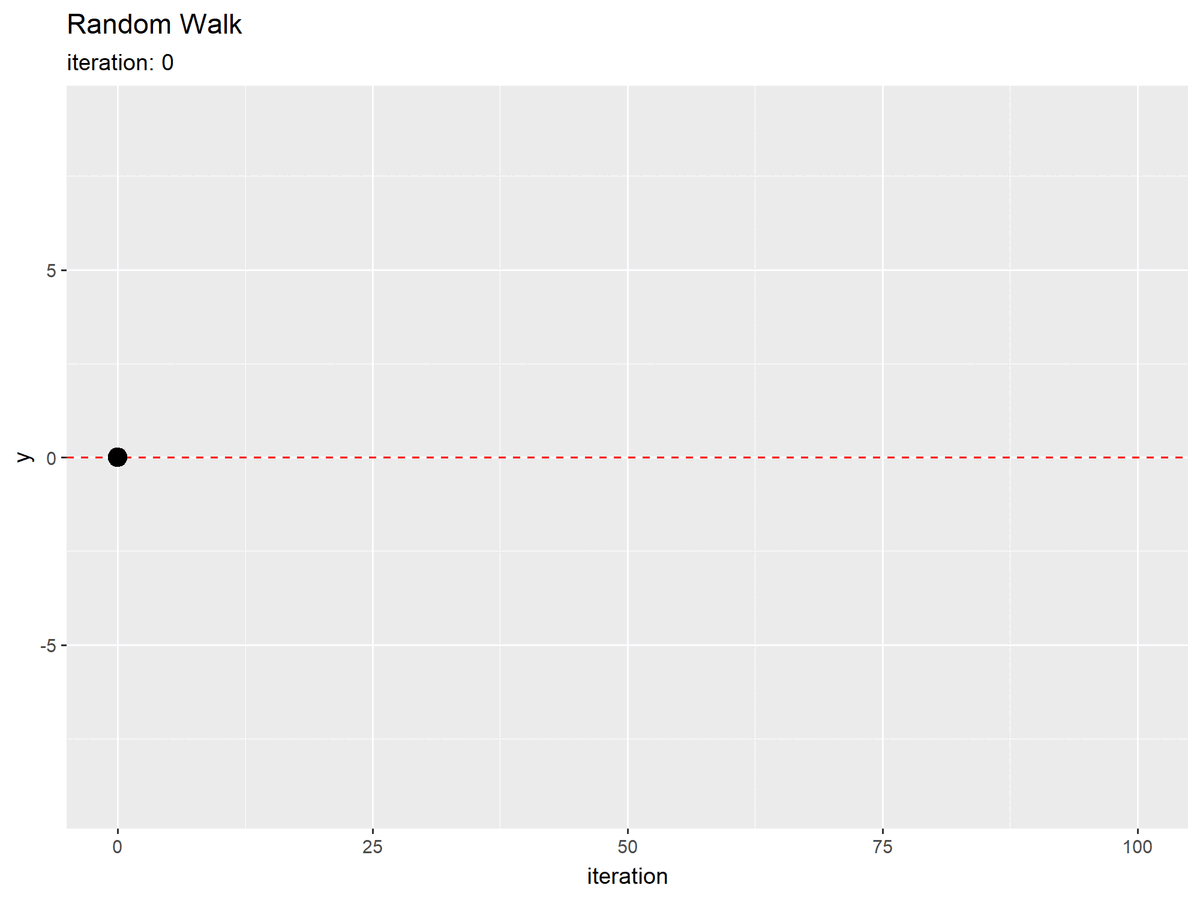
　初期値(期待値)を破線で示します。
　試行回数(時間)の変化を横軸で表しているので2次元に変化していますが、あくまで縦軸に対してランダムに移動しています。

複数サンプル

　続いて、複数のサンプルを並べて描画します。
　作図コードについては「GitHub - anemptyarchive/gganimate/.../RandomWalk.R」を参照してください。

・最終結果

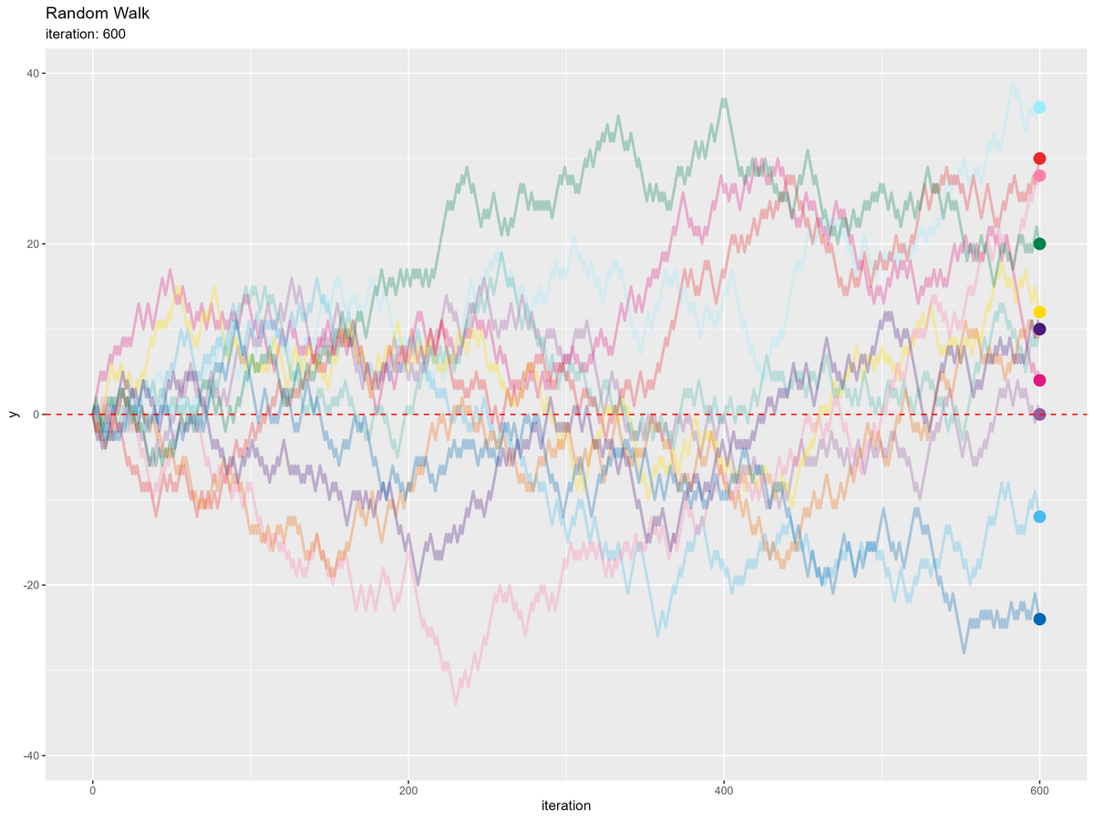
・推移のアニメーション

　等確率で移動する場合、初期値が期待値になりますが分散を持ち(散らばり)ます。

　この記事では、1次元の(上下に移動する)ランダムウォークを扱いました。次の記事では、2次元の(上下左右に移動する)場合を扱います。

おわりに

　transition_reveal()の記事の一部として書き始めたのですが、充実したので別の記事どころか3記事になりました。というわけで続きます。

2024.02.14：加筆修正しました。

　内容的には変わっていませんが、グラフの装飾周りが良くなりました。
　作業負荷(主に改修コスト)を下げるために、複数サンプルのコードを「解説はなしでGitHubを見てね」にしました。今後は他の記事でもこの形式でやっていくつもりです。

【次の内容】

からっぽのしょこ

読んだら書く！書いたら読む！同じ事は二度調べ(たく)ない

【R】1次元ランダムウォークの作図【gganimate】

はじめに

1次元ランダムウォークの作図

1サンプル

複数サンプル

おわりに