はじめに
『ゼロから作るDeep Learning 2――自然言語処理編』の初学者向け【実装】攻略ノートです。『ゼロつく2』学習の補助となるように適宜解説を加えています。本と一緒に読んでください。
本の内容を1つずつ確認しながらゆっくりと組んでいきます。
この記事は、7.4節「seq2seqの改良」の内容です。Encoderの隠れ状態を複数のレイヤに入力するPeeky seq2seqの処理を解説して、Pythonで実装します。
前項の記事とあわせて読んでください。
【前節の内容】
【他の節の内容】
【この節の内容】
7.4.1 入力データの反転(Reverse)
入力データの文字列を反転させることで、学習が良くなることがあります。
・スライス機能の確認
入力データの反転にはスライス機能を使います。簡単な配列を使ってスライス機能を確認しておきましょう。
# 1次元配列を作成
simple_x = np.arange(10)
print(simple_x)
[0 1 2 3 4 5 6 7 8 9]
変数名[l:m:n]でl番目以上でm番目未満の要素をn個間隔で取り出せます。
# スライス
print(simple_x[3:9:2])
[3 5 7]
1次元配列の変数に対して、変数名[::-1]とすることで配列を逆順に取り出せます(並び替えられます)。lとmを指定しないことで最初から最後までを表し、nが-1なことで後ろから1番目の要素を表します。
# 要素を反転
reverse_x = simple_x[::-1]
print(reverse_x)
[9 8 7 6 5 4 3 2 1 0]
2次元配列に対しても行ってみましょう。
# 2次元配列を作成
simple_x = np.arange(15).reshape((3, 5))
print(simple_x)
[[ 0  1  2  3  4]
 [ 5  6  7  8  9]
 [10 11 12 13 14]]
列のインデックスに対して1次元配列のときと同じ指定をすることで、列ごとに反転できます。
# 列を反転
reverse_x = simple_x[:, ::-1]
print(reverse_x)
[[ 4  3  2  1  0]
 [ 9  8  7  6  5]
 [14 13 12 11 10]]
これが足し算の式を表す文字列を逆順に並べ替えた状態です。
・seq2seqの評価(反転版)
Encoderの入力データ(足し算の式)を反転させて学習を行います。Decoderの入力データ(最後の文字を除いた足し算の答)と教師データ(最初の文字を除いた足し算の答)は反転しません。
# データを反転
reverse_x_train = x_train[:, ::-1]
reverse_x_test = x_test[:, ::-1]
print(''.join([id_to_char[c_id] for c_id in x_train[0]]))
print(''.join([id_to_char[c_id] for c_id in reverse_x_train[0]]))
71+118
 811+17
式を反転させるので、式と答は成り立たなくなります。しかし実際に計算するわけではなく、あくまで文字列(時系列データ)間のパターンをRNNで学習しています。
前項と同様にして、学習と評価を行います。
# インスタンスを作成
model = Seq2seq(vocab_size, wordvec_size, hidden_size)
optimizer = Adam()
trainer = Trainer(model, optimizer)

# 繰り返し試行
reverse_acc_list = []
for epoch in range(max_epoch):
    # 学習
    trainer.fit(reverse_x_train, t_train, max_epoch=1, batch_size=batch_size, max_grad=max_grad)

    # 正解数を初期化
    correct_num = 0

    # 精度を測定
    for n in range(len(reverse_x_test)):
        # データを取得
        question = reverse_x_test[[n]] # 入力データ(足し算の式)
        start_id = t_test[n, 0] # 区切り文字
        correct = t_test[n, 1:] # 教師データ(足し算の答)

        # 解答を生成
        guess = model.generate(question, start_id, len(correct))

        # 正解数をカウント
        if guess == list(correct): # 解答と答が一致したら
            correct_num += 1

    # 正解率を計算
    acc = float(correct_num) / len(reverse_x_test)
    reverse_acc_list.append(acc)

    # 途中経過を表示
    print('val acc:' + str(acc * 100))
| epoch 1 |  iter 1 / 351 | time 0[s] | loss 2.56
| epoch 1 |  iter 21 / 351 | time 0[s] | loss 2.52
| epoch 1 |  iter 41 / 351 | time 1[s] | loss 2.15
| epoch 1 |  iter 61 / 351 | time 1[s] | loss 1.94
| epoch 1 |  iter 81 / 351 | time 2[s] | loss 1.90
| epoch 1 |  iter 101 / 351 | time 3[s] | loss 1.86
| epoch 1 |  iter 121 / 351 | time 3[s] | loss 1.85
| epoch 1 |  iter 141 / 351 | time 4[s] | loss 1.84
| epoch 1 |  iter 161 / 351 | time 5[s] | loss 1.80
| epoch 1 |  iter 181 / 351 | time 5[s] | loss 1.78
| epoch 1 |  iter 201 / 351 | time 6[s] | loss 1.77
| epoch 1 |  iter 221 / 351 | time 7[s] | loss 1.76
| epoch 1 |  iter 241 / 351 | time 7[s] | loss 1.77
| epoch 1 |  iter 261 / 351 | time 8[s] | loss 1.76
| epoch 1 |  iter 281 / 351 | time 9[s] | loss 1.76
| epoch 1 |  iter 301 / 351 | time 9[s] | loss 1.75
| epoch 1 |  iter 321 / 351 | time 10[s] | loss 1.74
| epoch 1 |  iter 341 / 351 | time 11[s] | loss 1.73
val acc:0.27999999999999997
(省略)
| epoch 25 |  iter 261 / 351 | time 9[s] | loss 0.31
| epoch 25 |  iter 281 / 351 | time 9[s] | loss 0.31
| epoch 25 |  iter 301 / 351 | time 10[s] | loss 0.31
| epoch 25 |  iter 321 / 351 | time 11[s] | loss 0.30
| epoch 25 |  iter 341 / 351 | time 11[s] | loss 0.30
val acc:53.12
そのままの状態(前項)での正解率の推移と重ねてグラフにします。
# 正解率の記録をグラフ化
plt.figure(figsize=(9, 6))
plt.plot(1 + np.arange(len(acc_list)), acc_list,
         marker='o', label='baseline') # 素のままの入力データによる結果:7.3.4項
plt.plot(1 + np.arange(len(reverse_acc_list)), reverse_acc_list,
         marker='D', label='reverse') # 反転させた入力データによる結果
plt.xlabel('epoch')
plt.ylabel('accuracy')
plt.title('seq2seq', fontsize=20)
plt.ylim(0, 1) # y軸の表示範囲
plt.legend() # 凡例
plt.grid() # グリッド線
plt.show()
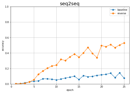
数式の文字列をそのまま入力したとき(baseline)よりも、反転して入力したとき(reverse)の方が正解率が上がっているのを確認できます。
この項では、seq2seqの学習をよくするために入力データを加工しました。次項では、seq2seq自体を改良します。
7.4.2 覗き見(Peeky)
7.3節で実装したseq2seqでは、EncoderからDecoderに入力する隠れ状態は、1つのLSTMレイヤに入力しました。この項で実装するPeeky版のseq2seqでは、Time LSTMレイヤとTime Affineレイヤに入力します。複数のレイヤに入力することによって、エンコードされた情報をより活用できることが期待できます。
・Peeky版のDecoderの処理の確認
図7-26を参考にして、Peeky版のDecoderの処理を確認していきます。共通する部分は省略するので、7.3節も参照してください。
・ネットワークの設定
まずは、RNNを構築します。
データとパラメータの形状に関する値を設定して、入力データ$\mathbf{xs} = (x_{0,0}, \cdots, x_{N-1,T-1})$を簡易的に作成します。
# データとパラメータの形状に関する値を指定
N = 6 # バッチサイズ
T = 4 # 時系列サイズ
V = 13 # 単語の種類数
D = 3 # 単語ベクトル(Embedレイヤの中間層)のサイズ
H = 5 # 隠れ状態(LSTMレイヤの中間層)のサイズ

# (簡易的に)入力データを作成
xs = np.random.randint(low=0, high=V, size=(N, T))
print(xs)
print(xs.shape)
[[10  4  2  2]
 [ 7 10  3  2]
 [10  0 11  7]
 [10  5  1  7]
 [ 1 12  8  4]
 [11  5  6 12]]
(6, 4)
各レイヤの重みとバイアスの初期値をランダムに生成します。
# Time Embedレイヤのパラメータを初期化
embed_W = (np.random.randn(V, D) * 0.01)

# Time LSTMレイヤのパラメータを初期化
lstm_Wx = (np.random.randn(H + D, 4 * H) / np.sqrt(H + D))
lstm_Wh = (np.random.randn(H, 4 * H) / np.sqrt(H))
lstm_b = np.zeros(4 * H).astype('f')

# Time Affineレイヤのパラメータを初期化
affine_W = (np.random.randn(H + H, V) / np.sqrt(H + H))
affine_b = np.zeros(V).astype('f')
Time LSTMレイヤとTime Affineレイヤには、これまでの入力とEncoderの隠れ状態$\mathbf{h}_{T-1}^{(\mathrm{Encoder})} = (h_{0,T-1,0}^{(\mathrm{Encoder})}, \cdots, h_{N-1,T-1,H-1}^{(\mathrm{Encoder})})$を結合したものが入力します。そのためTime LSTMレイヤとTime Affineレイヤの重みは、隠れ状態の次元数$H$分の行数が増えます。$\mathbf{h}_{T-1}^{(\mathrm{Encoder})}$の$T$はEncoderの時系列サイズです。
作成したパラメータを渡して、各レイヤのインスタンスを作成します。
# Time Embedレイヤのインスタンスを生成
embed_layer = TimeEmbedding(embed_W)

# Time Embedレイヤのインスタンスを生成
lstm_layer = TimeLSTM(lstm_Wx, lstm_Wh, lstm_b, stateful=True)

# Time Embedレイヤのインスタンスを生成
affine_layer = TimeAffine(affine_W, affine_b)
以上でRNNを構築できました。次は順伝播の処理を確認します。
・順伝播の計算
通常通り、xsをTime Embedレイヤに入力して、順伝播を計算します。
# Time Embedレイヤの順伝播を計算
xs = embed_layer.forward(xs)
print(np.round(xs[:, 0, :], 2))
print(xs.shape)
[[-0.   -0.    0.01]
 [ 0.    0.   -0.  ]
 [-0.   -0.    0.01]
 [-0.   -0.    0.01]
 [ 0.01  0.01 -0.01]
 [-0.01 -0.   -0.01]]
(6, 4, 3)
Time Embedレイヤに入力した$\mathbf{xs}$は、各要素が単語IDの2次元配列でした。Embedレイヤによって単語IDが単語ベクトルに変換され(3次元方向に拡張され)、3次元配列$\mathbf{xs} = (x_{0,0,0}, \cdots, x_{N-1,T-1,D-1})$になります。
TimeLSTMクラスのメソッドset_state()によって、Encoderの隠れ状態$\mathbf{h}_{T-1}^{(\mathrm{Encoder})}$をDecoderの0番目のLSTMレイヤに入力します。ここでは、$\mathbf{h}_{T-1}^{(\mathrm{Encoder})}$を簡易的に作成します。
# (簡易的に)Encoderからの入力を作成
encoder_h = np.random.randn(N, H)
print(np.round(encoder_h, 2))
print(encoder_h.shape)

# Encoderの隠れ状態を入力
lstm_layer.set_state(encoder_h)
[[ 0.78  0.65 -0.18 -0.2  -0.32]
 [ 0.02  0.3  -0.53  0.12 -1.27]
 [ 0.83  1.08 -0.14 -1.01  0.63]
 [ 0.94 -0.95 -0.55  0.01 -3.41]
 [ 0.05 -0.05  1.14  2.71  0.4 ]
 [ 0.5   0.24  0.46 -0.41 -1.25]]
(6, 5)
$\mathbf{h}_{T-1}^{(\mathrm{Encoder})}$をDecoderの時系列サイズ$T$個複製します。
# 時系列サイズ分に複製
encoder_hs = np.repeat(encoder_h, T, axis=0).reshape((N, T, H))
print(np.round(encoder_hs[:, T-1, :], 2))
print(encoder_hs.shape)
[[ 0.78  0.65 -0.18 -0.2  -0.32]
 [ 0.02  0.3  -0.53  0.12 -1.27]
 [ 0.83  1.08 -0.14 -1.01  0.63]
 [ 0.94 -0.95 -0.55  0.01 -3.41]
 [ 0.05 -0.05  1.14  2.71  0.4 ]
 [ 0.5   0.24  0.46 -0.41 -1.25]]
(6, 4, 5)
複製後の隠れ状態は、時刻方向に$T$次元増えて
$(N \times T \times H)$の3次元配列になります。
encoder_hs[:, t, :]のtを変えても、encoder_hと同じ配列になっているのを確認できます。
(ここでは登場しませんがEncoderの$T$(Encoderの時系列サイズ)個の隠れ状態$\mathbf{hs}^{(\mathrm{Encoder})} = (\mathbf{h}_0^{(\mathrm{Encoder})}, \cdots, \mathbf{h}_{T-1}^{(\mathrm{Encoder})})$とは別のものです。あくまで最後の$\mathbf{h}_{T-1}^{(\mathrm{Encoder})}$を$T$(Decoderの時系列サイズ)個に複製したものです。混同するようなら$\mathbf{hs}_{(T-1)}^{(\mathrm{Encoder})}$と表記したらいいかもしれません。)
「複製したEncoderの隠れ状態$\mathbf{hs}^{(\mathrm{Encoder})}$」と「Time Embedレイヤの出力$\mathbf{xs}$」を時刻ごとに行方向に結合します。
# 複製した隠れ状態とTime Embedレイヤの出力を結合
encoder_hs_xs = np.concatenate((encoder_hs, xs), axis=2)
print(np.round(encoder_hs_xs[:, 0, :], 2))
print(encoder_hs_xs.shape)
[[ 0.78  0.65 -0.18 -0.2  -0.32 -0.   -0.    0.01]
 [ 0.02  0.3  -0.53  0.12 -1.27  0.    0.   -0.  ]
 [ 0.83  1.08 -0.14 -1.01  0.63 -0.   -0.    0.01]
 [ 0.94 -0.95 -0.55  0.01 -3.41 -0.   -0.    0.01]
 [ 0.05 -0.05  1.14  2.71  0.4   0.01  0.01 -0.01]
 [ 0.5   0.24  0.46 -0.41 -1.25 -0.01 -0.   -0.01]]
(6, 4, 8)
結合した3次元配列から時刻$t$に関して取り出すと
$N$行$T + H$列の2次元配列です。
encoder_hs_xs[:, t, :]が、encoder_hs[:, t, :]とxs[:, t, :]を行方向に結合した配列になっているのを確認できます。
encoder_hs_xsをTime LSTMレイヤに入力して、順伝播を計算します。
# Time LSTMレイヤの順伝播を計算
decoder_hs = lstm_layer.forward(encoder_hs_xs)
print(np.round(decoder_hs[:, 0, :], 2))
print(decoder_hs.shape)
[[-0.1  -0.08  0.1  -0.1  -0.06]
 [ 0.03 -0.18  0.15 -0.06  0.05]
 [-0.13  0.06 -0.02 -0.05 -0.4 ]
 [ 0.14 -0.07  0.12 -0.    0.  ]
 [-0.18 -0.   -0.48  0.15 -0.01]
 [ 0.08 -0.16  0.21 -0.11  0.1 ]]
(6, 4, 5)
出力は、Decoderの隠れ状態$\mathbf{hs}^{(\mathrm{Decoder})} = (h_{0,0,0}^{(\mathrm{Decoder})}, \cdots, h_{N-1,T-1,H-1}^{(\mathrm{Decoder})})$です。
「複製したEncoderの隠れ状態$\mathbf{hs}^{(\mathrm{Encoder})}$」と「Decoderの隠れ状態$\mathbf{hs}^{(\mathrm{Decoder})}$」を時刻ごとに行方向に結合します。結合した配列を$\mathbf{hs} = (\mathbf{h}_0, \cdots, \mathbf{h}_{T-1})$とします。
# 複製したEncoderの隠れ状態とDecoderの隠れ状態を結合
hs = np.concatenate((encoder_hs, decoder_hs), axis=2)
print(np.round(hs[:, 0, :], 2))
print(hs.shape)
[[ 0.78  0.65 -0.18 -0.2  -0.32 -0.1  -0.08  0.1  -0.1  -0.06]
 [ 0.02  0.3  -0.53  0.12 -1.27  0.03 -0.18  0.15 -0.06  0.05]
 [ 0.83  1.08 -0.14 -1.01  0.63 -0.13  0.06 -0.02 -0.05 -0.4 ]
 [ 0.94 -0.95 -0.55  0.01 -3.41  0.14 -0.07  0.12 -0.    0.  ]
 [ 0.05 -0.05  1.14  2.71  0.4  -0.18 -0.   -0.48  0.15 -0.01]
 [ 0.5   0.24  0.46 -0.41 -1.25  0.08 -0.16  0.21 -0.11  0.1 ]]
(6, 4, 10)
$\mathbf{hs}$から時刻$t$に関して取り出すと
$N$行$H + H$列の2次元配列です。
hs[:, t, :]が、encoder_hs[:, t, :]とdecoder_hs[:, t, :]を行方向に結合した配列になっているのを確認できます。
hsをTime Affineレイヤに入力して、順伝播を計算します。
# Time Affineレイヤの順伝播を計算
score = affine_layer.forward(hs)
print(score.shape)
(6, 4, 13)
出力は、スコア$\mathbf{ys} = (y_{0,0,0}, \cdots, y_{N-1,T-1,V-1})$です。$\mathbf{ys}$をTime Softmax with Lossレイヤに入力して、損失$L$を計算します。
以上が順伝播の処理です。続いて、逆伝播の処理を確認します。
・逆伝播の計算
Time Softmax with LossレイヤからTime Affineレイヤに、$\mathbf{ys}$の勾配$\frac{\partial L}{\partial \mathbf{ys}} = \Bigl( \frac{\partial L}{\partial y_{0,0,0}}, \cdots, \frac{\partial L}{\partial y_{N-1,T-1,V-1}} \Bigr)$が入力します。
ここでは$\frac{\partial L}{\partial \mathbf{ys}}$を簡易的に作成して、逆伝播を計算します。
# (簡易的に)スコアの勾配を作成
dscore = np.random.randn(N, T, V)
print(dscore.shape)

# Time Affineレイヤの逆伝播を計算
dhs = affine_layer.backward(dscore)
print(np.round(dhs[:, 0, :], 2))
print(dhs.shape)
(6, 4, 13)
[[-0.98  0.65 -0.75  0.87 -0.38 -0.16  1.41 -0.59 -0.02 -0.79]
 [-1.63 -0.04  0.92  1.41 -0.51 -1.55  0.93 -0.26 -0.5   0.69]
 [ 0.12 -1.13 -0.02  1.16 -0.9  -2.08  2.02  1.62 -0.15  1.95]
 [-1.35 -0.71 -2.05  0.63  0.36  1.49 -0.1  -1.21  1.75  1.39]
 [-0.1  -0.39  2.3   0.59  0.37 -1.27 -0.2   0.08 -1.03 -0.53]
 [ 1.5  -0.05 -1.28 -1.84  0.26  1.13 -1.52  0.29  0.26 -1.37]]
(6, 4, 10)
出力は、$\mathbf{hs}$の勾配$\frac{\partial L}{\partial \mathbf{hs}} = \Bigl( \frac{\partial L}{\partial \mathbf{h}_0}, \cdots, \frac{\partial L}{\partial \mathbf{h}_{T-1}} \Bigr)$です。$\frac{\partial L}{\partial \mathbf{hs}}$から時刻$t$に関して取り出すと
$N$行$H + H$の2次元配列です。
$\frac{\partial L}{\partial \mathbf{hs}}$を「複製したEncoderの隠れ状態の勾配$\frac{\partial L}{\partial \mathbf{hs}^{(\mathrm{Encoder})}}$」と「Decoderの隠れ状態の勾配$\frac{\partial L}{\partial \mathbf{hs}^{(\mathrm{Decoder})}}$」に分割します。
# 複製したEncoderの隠れ状態の勾配を分割
encoder_dhs0 = dhs[:, :, :H]
print(np.round(encoder_dhs0[:, 0, :], 2))
print(encoder_dhs0.shape)

# Decoderの隠れ状態の勾配を分割
decoder_dhs = dhs[:, :, H:]
print(np.round(decoder_dhs[:, 0, :], 2))
print(decoder_dhs.shape)
[[-0.98  0.65 -0.75  0.87 -0.38]
 [-1.63 -0.04  0.92  1.41 -0.51]
 [ 0.12 -1.13 -0.02  1.16 -0.9 ]
 [-1.35 -0.71 -2.05  0.63  0.36]
 [-0.1  -0.39  2.3   0.59  0.37]
 [ 1.5  -0.05 -1.28 -1.84  0.26]]
(6, 4, 5)
[[-0.16  1.41 -0.59 -0.02 -0.79]
 [-1.55  0.93 -0.26 -0.5   0.69]
 [-2.08  2.02  1.62 -0.15  1.95]
 [ 1.49 -0.1  -1.21  1.75  1.39]
 [-1.27 -0.2   0.08 -1.03 -0.53]
 [ 1.13 -1.52  0.29  0.26 -1.37]]
(6, 4, 5)
$\frac{\partial L}{\partial \mathbf{hs}^{(\mathrm{Encoder})}}$と$\frac{\partial L}{\partial \mathbf{hs}^{(\mathrm{Decoder})}}$からそれぞれ時刻$t$に関して取り出すと
どちらも$N$行$H$列の2次元配列です。
dhs[:, t, :]が、encoder_dhs0[:, t, :]とdecoder_dhs[:, t, :]を行方向に結合した配列になっているのを確認できます。
$\frac{\partial L}{\partial \mathbf{hs}^{(\mathrm{Decoder})}}$をTime LSTMレイヤに入力して、逆伝播を計算します。
# Time LSTMレイヤの逆伝播を計算
encoder_dhs_dxs = lstm_layer.backward(decoder_dhs)
print(np.round(encoder_dhs_dxs[:, 0, :], 2))
print(encoder_dhs_dxs.shape)
[[-0.03 -0.2  -0.12  0.1  -0.01  0.11 -0.06  0.07]
 [ 0.02 -0.21 -0.35  0.29  0.06  0.18 -0.01  0.17]
 [ 0.43 -0.05 -0.33 -0.2  -0.01 -0.17  0.08  0.14]
 [ 0.05 -0.08 -0.1  -0.07  0.06  0.05 -0.03 -0.04]
 [ 0.09  0.06 -0.08 -0.04  0.    0.03 -0.16 -0.12]
 [ 0.13  0.3  -0.02 -0.08  0.19 -0.04 -0.16 -0.09]]
(6, 4, 8)
出力した3次元配列から時刻$t$に関して取り出すと
$N$行$H + D$列の2次元配列です。
これを「複製したEncoderの隠れ状態の勾配$\frac{\partial L}{\partial \mathbf{hs}^{(\mathrm{Encoder})}}$」と「Time Embedレイヤの出力の勾配$\frac{\partial L}{\partial \mathbf{xs}}$」に分割します。
# 複製したEncoderの隠れ状態の勾配を分割
encoder_dhs1 = encoder_dhs_dxs[:, :, :H]
print(np.round(encoder_dhs1[:, 0, :], 2))
print(encoder_dhs1.shape)

# Time Embedの入力の勾配を分割
dxs = encoder_dhs_dxs[:, :, H:]
print(np.round(dxs[:, 0, :], 2))
print(dxs.shape)
[[-0.03 -0.2  -0.12  0.1  -0.01]
 [ 0.02 -0.21 -0.35  0.29  0.06]
 [ 0.43 -0.05 -0.33 -0.2  -0.01]
 [ 0.05 -0.08 -0.1  -0.07  0.06]
 [ 0.09  0.06 -0.08 -0.04  0.  ]
 [ 0.13  0.3  -0.02 -0.08  0.19]]
(6, 4, 5)
[[ 0.11 -0.06  0.07]
 [ 0.18 -0.01  0.17]
 [-0.17  0.08  0.14]
 [ 0.05 -0.03 -0.04]
 [ 0.03 -0.16 -0.12]
 [-0.04 -0.16 -0.09]]
(6, 4, 3)
$\frac{\partial L}{\partial \mathbf{hs}^{(\mathrm{Encoder})}}$から時刻$t$に関して取り出すと
$N$行$H$列の2次元配列です。もう一方は、$\frac{\partial L}{\partial \mathbf{xs}} = \Bigl( \frac{\partial L}{\partial x_{0,0,0}}, \cdots, \frac{\partial L}{\partial x_{N-1,T-1,D-1}} \Bigr)$です。
$\frac{\partial L}{\partial \mathbf{xs}}$をTime Embedレイヤに入力して、逆伝播を計算します。
# Time Embedレイヤの逆伝播を計算
dout = embed_layer.backward(dxs)
print(dout)
None
Time Embedレイヤより先はないので、Noneを返します。入力データの勾配は返しません。
複製したEncoderの隠れ状態$\mathbf{hs}^{(\mathrm{Encoder})}$の勾配が「Time Affineレイヤの出力から取り出した$\frac{\partial L}{\partial \mathbf{hs}^{(\mathrm{Encoder})}}$」と「Time LSTMレイヤの出力から取り出した$\frac{\partial L}{\partial \mathbf{hs}^{(\mathrm{Encoder})}}$」の2つ得られました。これは$\mathbf{hs}^{(\mathrm{Encoder})}$が分岐して順伝播したためです。
分岐ノードの逆伝播では、2つの勾配の和を計算します(1.3.4.2項「分岐ノード」)。
# 分岐した2つの「複製したEncoderの隠れ状態の勾配」の和を計算
encoder_dhs = encoder_dhs0 + encoder_dhs1
print(encoder_dhs.shape)
(6, 4, 5)
分岐した勾配の和が、最終的な複製したEncoderの隠れ状態$\mathbf{hs}^{(\mathrm{Encoder})}$の勾配$\frac{\partial L}{\partial \mathbf{hs}^{(\mathrm{Encoder})}}$です。
同様に、Encoderの隠れ状態$\mathbf{h}_{T-1}^{(\mathrm{Encoder})}$(の各要素)も$T$個に分岐したのでした。
これについても全ての和をとる必要があります(1.3.4.3項「Repeatノード」)。
# 分岐したT個の「Encoderの隠れ状態の勾配」の和を計算
sum_encoder_dhs = np.sum(encoder_dhs, axis=1)
print(sum_encoder_dhs.shape)
(6, 5)
えーとまだあります。
最初に$\mathbf{h}_{T-1}^{(\mathrm{Encoder})}$がDecoderの0番目のLSTMレイヤに入力していたのを思い出してください。それも加える必要があります。
その勾配は、TimeLSTMクラスの逆伝播メソッドbackward()の実行時に計算され、インスタンス変数dhに保存されています。これを先ほどの$T$個分の和sum_encoder_dhsに加えます。
# EncoderのT-1番目の隠れ状態の勾配を計算
dh = lstm_layer.dh + sum_encoder_dhs
print(np.round(dh, 2))
print(dh.shape)
[[-3.87 -5.11  3.52  8.2  -1.9 ]
 [ 1.75  1.95 -2.11  1.06 -2.37]
 [ 1.9  -1.97 -1.23  0.57 -3.52]
 [-3.19 -2.59 -0.42  2.64 -1.21]
 [-1.05 -2.46  2.98  3.21 -1.1 ]
 [ 9.63  8.36  0.05 -4.54  8.15]]
(6, 5)
これで分岐した全ての勾配の和が求まりました。これが最終的なEncoderの隠れ状態$\mathbf{h}_{T-1}^{(\mathrm{Encoder})}$の勾配$\frac{\partial L}{\partial \mathbf{h}_{T-1}^{(\mathrm{Encoder})}}$です。
$\frac{\partial L}{\partial \mathbf{h}_{T-1}}$をEncoderの$T-1$番目のLSTMレイヤに入力します。
以上が学習時に行う処理です。
・文章生成
文章(足し算の解答)を生成する処理については、基本的に7.3.3項のseq2seqのときと同じです。順伝播の処理での変更点である入力データを結合する処理が追加されています。
・Peeky版のDecoderの実装
処理の確認ができたので、Peeky Decoderをクラスとして実装します。
# Peeky版のデコーダーの実装
class PeekyDecoder:
    # 初期化メソッド
    def __init__(self, vocab_size, wordvec_size, hidden_size):
        # 変数の形状に関する値を取得
        V, D, H = vocab_size, wordvec_size, hidden_size

        # パラメータを初期化
        embed_W = (np.random.randn(V, D) * 0.01).astype('f')
        lstm_Wx = (np.random.randn(H + D, 4 * H) / np.sqrt(H + D)).astype('f')
        lstm_Wh = (np.random.randn(H, 4 * H) / np.sqrt(H)).astype('f')
        lstm_b = np.zeros(4 * H).astype('f')
        affine_W = (np.random.randn(H + H, V) / np.sqrt(H + H)).astype('f')
        affine_b = np.zeros(V).astype('f')

        # レイヤを生成
        self.embed = TimeEmbedding(embed_W)
        self.lstm = TimeLSTM(lstm_Wx, lstm_Wh, lstm_b, stateful=True)
        self.affine = TimeAffine(affine_W, affine_b)

        # パラメータと勾配をリストに格納
        self.params = [] # パラメータ
        self.grads = []  # 勾配
        for layer in (self.embed, self.lstm, self.affine):
            self.params += layer.params
            self.grads += layer.grads

        # 中間変数の受け皿
        self.cache = None

    # 順伝播メソッド
    def forward(self, xs, h):
        # 変数の形状に関する値を取得
        N, T = xs.shape
        N, H = h.shape

        # Encoderの隠れ状態を入力
        self.lstm.set_state(h)

        # Time Embedレイヤの順伝播を計算
        out = self.embed.forward(xs)

        # Encoderの隠れ状態を複製
        hs = np.repeat(h, T, axis=0).reshape((N, T, H))

        # Encoderの隠れ状態(複製)と単語ベクトルを結合
        out = np.concatenate((hs, out), axis=2)

        # Time LSTMレイヤの順伝播を計算
        out = self.lstm.forward(out)

        # Encoderの隠れ状態(複製)とDecoderの隠れ状態を結合
        out = np.concatenate((hs, out), axis=2)

        # Time Affineレイヤの順伝播を計算
        score = self.affine.forward(out)

        # 逆伝播用に値を保存
        self.cache = H
        return score

    # 逆伝播メソッド
    def backward(self, dscore):
        # 変数の形状に関する値を取得
        H = self.cache

        # Time Affineレイヤの逆伝播を計算
        dout = self.affine.backward(dscore)

        # 勾配を分割
        dhs0 = dout[:, :, :H] # Encoderの隠れ状態(複製)の勾配
        dout = dout[:, :, H:] # Decoderの隠れ状態の勾配

        # Time LSTMレイヤの逆伝播を計算
        dout = self.lstm.backward(dout)

        # 勾配を分割
        dhs1 = dout[:, :, :H]   # Encoderの隠れ状態(複製)の勾配
        dembed = dout[:, :, H:] # 単語ベクトルの勾配

        # Time Embedレイヤの逆伝播を計算
        dout = self.embed.backward(dembed) # 返り値はNone

        # Encoderの隠れ状態の勾配を計算
        dhs = dhs0 + dhs1 # Encoderの隠れ状態(複製)の勾配を合算
        dh = self.lstm.dh + np.sum(dhs, axis=1) # EncoderのT-1番目の隠れ状態の勾配を合算
        return dh

    # 文章生成メソッド
    def generate(self, h, start_id, sample_size):
        # 文字IDの受け皿を初期化
        sampled = []

        # 区切り文字のIDを設定
        char_id = start_id

        # エンコードされた足し算の式を入力
        self.lstm.set_state(h)

        # 解答を生成
        H = h.shape[1]
        peeky_h = h.reshape((1, 1, H))
        for _ in range(sample_size):
            # 入力用に2次元配列に変換
            x = np.array([char_id]).reshape((1, 1))

            # 単語ベクトルを計算
            out = self.embed.forward(x)

            # 隠れ状態を計算
            out = np.concatenate((peeky_h, out), axis=2)
            out = self.lstm.forward(out)

            # スコアを計算
            out = np.concatenate((peeky_h, out), axis=2)
            score = self.affine.forward(out)

            # スコアが最大の文字IDを取得
            char_id = np.argmax(score.flatten()) # 入力データを更新
            sampled.append(char_id) # サンプルを保存

        return sampled
TimeEmbedクラスの逆伝播メソッドbackward()はNoneを返します。よって、Encoderの逆伝播メソッドbackward()もNoneを返します。
実装したクラスを試してみましょう。
簡易的な入力データ$\mathbf{xs}$と、PeekyDecoderのインスタンスを作成します。
# (簡易的に)入力データを作成
xs = np.random.randint(low=0, high=V, size=(N, T))
print(xs)
print(xs.shape)

# Decoderのインスタンスを作成
decoder = PeekyDecoder(V, D, H)
[[ 5 12  1  3]
 [ 1  5  0  6]
 [ 9  8  6  6]
 [10  3 10  0]
 [10  8  3  6]
 [ 3  9  4 11]]
(6, 4)
簡易的にEncoderの隠れ状態$\mathbf{h}_{T-1}$を作成して、順伝播を計算します。
# (簡易的に)Encoderからの入力を作成
h = np.random.randn(N, H)
print(h.shape)

# Decoderの順伝播を計算
score = decoder.forward(xs, h)
print(np.round(score[:, 0, :], 2))
print(score.shape)
(6, 5)
[[ 0.32 -0.05 -0.91 -0.67  0.11 -0.92  0.2   0.25  0.54  0.98 -0.02  0.26
  -0.19]
 [-0.48 -0.57  0.45 -0.86  0.87 -0.15  1.67  1.18  0.62 -0.43 -1.75  0.87
   0.22]
 [ 1.28  0.08  0.18  0.24 -0.22 -0.33 -0.82 -0.34  0.05  0.3   0.74 -0.1
  -1.29]
 [ 0.25  0.51  0.68  0.17 -0.21 -0.06 -0.08 -0.63  0.2  -0.35  0.5  -0.03
  -0.59]
 [ 0.48 -1.44 -2.58 -0.37  0.59 -0.78 -0.56  1.54 -0.33  1.74 -0.67  0.18
   0.4 ]
 [-0.64  1.2  -0.02 -0.94 -0.32  0.09  0.55 -0.37  0.87  1.23 -0.16 -0.64
   1.54]]
(6, 4, 13)
Decoderの入力データ$\mathbf{xs}$とエンコードされたEncoderの入力情報$\mathbf{h}_{T-1}$から、スコア$\mathbf{ys}$が得られました。$\mathbf{ys}$は、Time Softmax with Lossレイヤに入力して損失$L$を求めます。
続いて、逆伝播の入力(Time Softmax with Lossレイヤの出力)$\frac{\partial L}{\partial \mathbf{ys}}$を簡易的に作成して、逆伝播の計算を行います。
# (簡易的に)スコアの勾配を作成
dscore = np.ones((N, T, V))
print(dscore.shape)

# 逆伝播を計算
dh = decoder.backward(dscore)
print(np.round(dh, 2))
print(dh.shape)
(6, 4, 13)
[[ 2.7   5.71  0.05  5.53  0.12]
 [ 2.27  5.74  0.1   5.06  0.05]
 [ 2.52  5.17  0.29  5.4   0.29]
 [ 2.82  5.02  0.3   5.24  0.38]
 [ 2.11  5.53  0.18  5.3  -0.65]
 [ 2.58  4.9   0.51  4.51 -0.12]]
(6, 5)
各レイヤのパラメータの勾配が得られました。勾配情報は、インスタンス内に保持されています。確率的勾配降下法を用いてパラメータを更新します。
また、Encoderの隠れ状態の勾配$\frac{\partial L}{\partial \mathbf{h}_0}$をEncoderの$T-1$番目のLSTMレイヤに入力します。
最後に、文章生成を行います。
# 最初に入力する単語のIDを指定
start_id = 6

# (簡易的に)Encoderからの入力を作成
h = np.random.randn(1, H)
print(h.shape)

# 文章を生成
sampled = decoder.generate(h, start_id, T)
print(sampled)
print(''.join([id_to_char[c_id] for c_id in sampled]))
(1, 5)
[2, 2, 2, 2]
++++
学習を行っていないので、結果はデタラメです。また、文字列への変換に利用するid_to_charは7.2.4項の足し算データセットを読み込む必要があります。
以上でPeeky版のDecoderを実装できました。次は、Peeky Decoderを利用してPeeky版のseq2seqを実装します。
・Peeky版のseq2seqの実装
7.3.3項で実装したseq2seqとの違いは、デコーダーにPeekyDecoderを使うところだけです。よってSeq2seqクラスを継承して、初期化メソッドのみを書き換えることで実装します。
# Peeky版のseq2seqの実装
class PeekySeq2seq(Seq2seq):
    # 初期化メソッド
    def __init__(self, vocab_size, wordvec_size, hidden_size):
        # 変数の形状に関する値を取得
        V, D, H = vocab_size, wordvec_size, hidden_size

        # 各レイヤのインスタンスを作成
        self.encoder = Encoder(V, D, H)
        self.decoder = PeekyDecoder(V, D, H)
        self.softmax = TimeSoftmaxWithLoss()

        # パラメータと勾配をリストに格納
        self.params = self.encoder.params + self.decoder.params
        self.grads = self.encoder.grads + self.decoder.grads
PeekyDecoderのインスタンス名をSeq2seqのときと同じdecoderとすることで、他のメソッドはそのまま利用できます。
・Peeky seq2seqの評価
これまでと同様にして、Peeky版のseq2seqの学習を行います。学習には、足し算データセット(7.2.4項)を反転させたものを利用します。
# インスタンスを作成
model = PeekySeq2seq(vocab_size, wordvec_size, hidden_size)
optimizer = Adam()
trainer = Trainer(model, optimizer)

# 繰り返し試行
peeky_reverse_acc_list = []
for epoch in range(max_epoch):
    # 学習
    trainer.fit(reverse_x_train, t_train, max_epoch=1, batch_size=batch_size, max_grad=max_grad)

    # 正解数を初期化
    correct_num = 0

    # 精度を測定
    for n in range(len(reverse_x_test)):
        # データを取得
        question = reverse_x_test[[n]]  # 入力データ(足し算の式)
        start_id = t_test[n, 0] # 区切り文字
        correct = t_test[n, 1:] # 教師データ(足し算の答)

        # 解答を生成
        guess = model.generate(question, start_id, len(correct))

        # 正解数をカウント
        if guess == list(correct): # 解答と答が一致したら
            correct_num += 1

    # 正解率を計算
    acc = float(correct_num) / len(reverse_x_test)
    peeky_reverse_acc_list.append(acc)

    # 途中経過を表示
    print('val acc:' + str(acc * 100))
| epoch 1 |  iter 1 / 351 | time 0[s] | loss 2.56
| epoch 1 |  iter 21 / 351 | time 0[s] | loss 2.46
| epoch 1 |  iter 41 / 351 | time 1[s] | loss 2.17
| epoch 1 |  iter 61 / 351 | time 2[s] | loss 1.97
| epoch 1 |  iter 81 / 351 | time 2[s] | loss 1.90
| epoch 1 |  iter 101 / 351 | time 3[s] | loss 1.83
| epoch 1 |  iter 121 / 351 | time 4[s] | loss 1.80
| epoch 1 |  iter 141 / 351 | time 5[s] | loss 1.79
| epoch 1 |  iter 161 / 351 | time 5[s] | loss 1.78
| epoch 1 |  iter 181 / 351 | time 6[s] | loss 1.77
| epoch 1 |  iter 201 / 351 | time 7[s] | loss 1.77
| epoch 1 |  iter 221 / 351 | time 8[s] | loss 1.77
| epoch 1 |  iter 241 / 351 | time 8[s] | loss 1.75
| epoch 1 |  iter 261 / 351 | time 9[s] | loss 1.75
| epoch 1 |  iter 281 / 351 | time 10[s] | loss 1.75
| epoch 1 |  iter 301 / 351 | time 11[s] | loss 1.73
| epoch 1 |  iter 321 / 351 | time 11[s] | loss 1.72
| epoch 1 |  iter 341 / 351 | time 12[s] | loss 1.72
val acc:0.16
(省略)
| epoch 25 |  iter 261 / 351 | time 9[s] | loss 0.03
| epoch 25 |  iter 281 / 351 | time 10[s] | loss 0.03
| epoch 25 |  iter 301 / 351 | time 11[s] | loss 0.04
| epoch 25 |  iter 321 / 351 | time 11[s] | loss 0.02
| epoch 25 |  iter 341 / 351 | time 12[s] | loss 0.02
val acc:96.61999999999999
これまでの結果と重ねて可視化します。
# 正解率の記録をグラフ化
plt.figure(figsize=(9, 6))
plt.plot(1 + np.arange(len(acc_list)), acc_list,
         marker='o', label='baseline') # 素のままの入力データによる結果:7.3.4項
plt.plot(1 + np.arange(len(reverse_acc_list)), reverse_acc_list,
         marker='D', label='reverse') # 反転させた入力データによる結果:7.4.1項
plt.plot(1 + np.arange(len(peeky_reverse_acc_list)), peeky_reverse_acc_list,
         marker='v', label='reverse + peeky') # 反転させた入力データによるPeeky版の結果
plt.xlabel('epoch')
plt.ylabel('accuracy')
plt.title('seq2seq', fontsize=20)
plt.ylim(0, 1) # y軸の表示範囲
plt.legend() # 凡例
plt.grid() # グリッド線
plt.show()
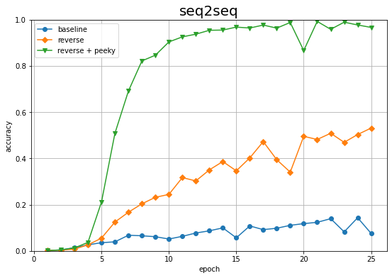
素のままの推移(baseline)と入力データを反転させた推移(reverse)よりも高くなりました。少ないエポック数で正解率が100%近くまで上がっています。
折角なので、反転しない足し算の式を使ったPeeky版のseq2seqの評価も見てみましょう。
# インスタンスを作成
model = PeekySeq2seq(vocab_size, wordvec_size, hidden_size)
optimizer = Adam()
trainer = Trainer(model, optimizer)

# 繰り返し試行
peeky_acc_list = []
for epoch in range(max_epoch):
    # 学習
    trainer.fit(x_train, t_train, max_epoch=1, batch_size=batch_size, max_grad=max_grad)

    # 正解数を初期化
    correct_num = 0

    # 精度を測定
    for n in range(len(x_test)):
        # データを取得
        question = x_test[[n]]  # 入力データ(足し算の式)
        start_id = t_test[n, 0] # 区切り文字
        correct = t_test[n, 1:] # 教師データ(足し算の答)

        # 解答を生成
        guess = model.generate(question, start_id, len(correct))

        # 正解数をカウント
        if guess == list(correct): # 解答と答が一致したら
            correct_num += 1

    # 正解率を計算
    acc = float(correct_num) / len(x_test)
    peeky_acc_list.append(acc)

    # 途中経過を表示
    print('val acc:' + str(acc * 100))
| epoch 1 |  iter 1 / 351 | time 0[s] | loss 2.56
| epoch 1 |  iter 21 / 351 | time 0[s] | loss 2.47
| epoch 1 |  iter 41 / 351 | time 1[s] | loss 2.18
| epoch 1 |  iter 61 / 351 | time 2[s] | loss 1.96
| epoch 1 |  iter 81 / 351 | time 2[s] | loss 1.86
| epoch 1 |  iter 101 / 351 | time 3[s] | loss 1.82
| epoch 1 |  iter 121 / 351 | time 4[s] | loss 1.79
| epoch 1 |  iter 141 / 351 | time 4[s] | loss 1.78
| epoch 1 |  iter 161 / 351 | time 5[s] | loss 1.77
| epoch 1 |  iter 181 / 351 | time 6[s] | loss 1.77
| epoch 1 |  iter 201 / 351 | time 6[s] | loss 1.77
| epoch 1 |  iter 221 / 351 | time 7[s] | loss 1.76
| epoch 1 |  iter 241 / 351 | time 8[s] | loss 1.76
| epoch 1 |  iter 261 / 351 | time 9[s] | loss 1.75
| epoch 1 |  iter 281 / 351 | time 9[s] | loss 1.75
| epoch 1 |  iter 301 / 351 | time 10[s] | loss 1.75
| epoch 1 |  iter 321 / 351 | time 11[s] | loss 1.74
| epoch 1 |  iter 341 / 351 | time 11[s] | loss 1.74
val acc:0.18
(省略)
| epoch 25 |  iter 261 / 351 | time 9[s] | loss 0.34
| epoch 25 |  iter 281 / 351 | time 10[s] | loss 0.34
| epoch 25 |  iter 301 / 351 | time 11[s] | loss 0.35
| epoch 25 |  iter 321 / 351 | time 11[s] | loss 0.38
| epoch 25 |  iter 341 / 351 | time 12[s] | loss 0.37
val acc:37.24
推移を見ます。
# 正解率の記録をグラフ化
plt.figure(figsize=(9, 6))
plt.plot(1 + np.arange(len(acc_list)), acc_list,
         marker='o', label='baseline') # 素のままの入力データによる結果:7.3.4項
plt.plot(1 + np.arange(len(reverse_acc_list)), reverse_acc_list,
         marker='D', label='reverse') # 反転させた入力データによる結果:7.4.1項
plt.plot(1 + np.arange(len(peeky_reverse_acc_list)), peeky_reverse_acc_list,
         marker='v', label='reverse + peeky') # 反転させた入力データによるPeeky版の結果
plt.plot(1 + np.arange(len(peeky_acc_list)), peeky_acc_list,
         marker='^', label='peeky') # 素のままの入力データによるPeeky版の結果
plt.xlabel('epoch')
plt.ylabel('accuracy')
plt.title('seq2seq', fontsize=20)
plt.ylim(0, 1) # y軸の表示範囲
plt.legend() # 凡例
plt.grid() # グリッド線
plt.show()

この例では、Peekyよりも入力データの反転の方が効果があるようです。
以上で7章の内容は完了です。次章では、Attentionというメカニズムを導入して、seq2seqをさらに改善します。
参考文献

おわりに
7章完了!LSTMレイヤそのものに比べれば難しくはないですが、言葉で説明するのに非常に苦労しました。まぁ苦労した分理解は深まるのですがね。でもコスパはなんとも言えない。
そんなこんなで少しは理解が進んだので、1巻の記事から全部加筆修正したーい、年度内に2巻終わらせたーい、3巻も買っちゃったので早くやりたーい。
【次節の内容】
つづく